USA USAAIO 2026 · Correction by IOAI Training

Mixed Functions Parameter Regression

This page gives the full approach. Read it once you have searched.

Metric: RMSE over all parameters
Evaluated on: held-out validation (official test labels are private)
Our score: RMSE 0.0555 on 400 train groups
Expected level: beat k-means baseline (our run: 1.009 clipped)

Expected level reached

We solved the problem ourselves: downloaded the data, ran the experiments and measured the score below. The statement and data belong to their organisers.

The problem in brief

Each "group" is a cloud of 400 points $(x, y)$ in random order. Behind every group hide four curves, 100 points each: an exponential $a_0 e^{a_1 x} + a_2$ , a logarithm $b_0 \ln x + b_1$ , a sinusoid $c_0 \sin(c_1 x + c_2) + c_3$ and a line $d_0 x + d_1$ , all with Gaussian noise added to $y$ . Nobody tells you which point belongs to which curve. From the 400 points you must recover all 11 parameters. You get 400 training groups with their true parameters and must predict the parameters of 200 test groups. It is a regression problem in disguise: the real difficulty is the missing labels, which turns it into an unsupervised mixture of regressions.

How you are scored

The metric is the root mean squared error over every predicted parameter of every test group,

\text{RMSE} = \sqrt{\frac{1}{N}\sum_{i=1}^{N}(\hat p_i - p_i)^2}, \qquad N = 11 \times 200 .

The organisers define a baseline (k-means with $k = 4$ on the points, then fit every family on every cluster and keep the best fit per family), and the final score is $\frac{X_{\text{baseline}} - X}{X_{\text{baseline}} - X_{\text{best}}}\times 100\%$ , where $X_{\text{best}}$ is the best contestant's RMSE. Neither $X_{\text{baseline}}$ nor $X_{\text{best}}$ is published, and the test parameters are private, so all numbers below are measured on the 400 training groups, whose true parameters are given. Our method learns only a handful of global constants from them (the parameter ranges, the $x$ ranges, the noise level), so this validation is honest up to those 15 or so numbers.

First look at the data

Plotting a few groups and comparing with the training parameters reveals a lot of structure that the statement does not spell out:

Every family lives on its own $x$ interval. A histogram of all $x$ values is piecewise flat, and the jumps sit at $-3$ , $0$ , $0.5$ , about $1.1$ , $5$ , $10$ and $4\pi$ . Matching levels gives: line on $[-3, 5]$ , exponential on $[0.5, 5]$ , log on $[1.1, 10]$ , sine on $[0, 4\pi]$ , each uniform. So a point with $x < 0$ is surely on the line, and a point with $x > 10$ surely on the sine.
The parameters are uniform in a box: $a_0 \in [0.5, 3]$ , $a_1 \in [0.1, 0.8]$ , $a_2 \in [-0.5, 0.5]$ , $b_0 \in [0.5, 3]$ , $b_1 \in [-1, 1]$ , $c_0 \in [1, 3]$ , $c_1 \in [0.5, 2]$ , $c_2 \in [-1, 1]$ , $c_3 \in [0, 2]$ , $d_0 \in [0.3, 1.5]$ , $d_1 \in [-2, 2]$ .
The noise is Gaussian with $\sigma \approx 0.12$ , the same in every group (measured on the points with $x < 0$ and $x > 10$ , whose family is known; kurtosis 2.98, close to the Gaussian 3).

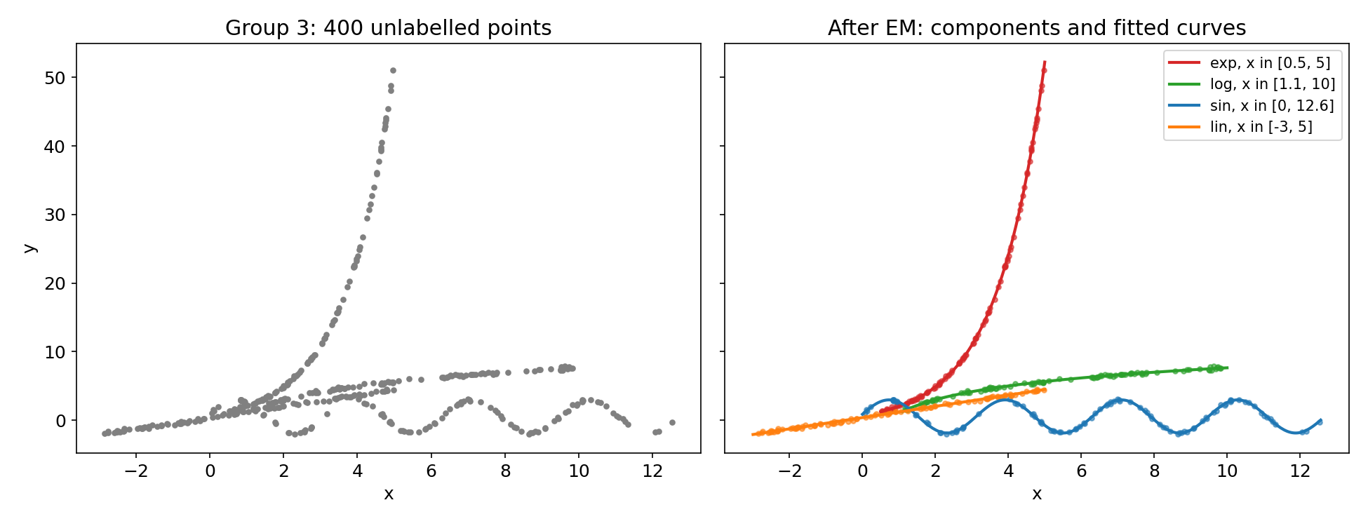
Left: the 400 points of one training group, unlabelled: an exponential shooting up to y = 50 near x = 5, a slowly rising log curve, a sine wave between -2 and 3, and a straight line, all crossing near x between 0 and 3. Right: the same points coloured by the component our EM assigns them to, with the four fitted curves drawn over their own x-ranges.

The curves cross each other in the region $x \in [0.5, 3]$ , where all four families are active and where most of the ambiguity lies.

A first baseline

Predicting the centre of every parameter box gives RMSE 0.621: that is the "know nothing" level. The organisers' k-means baseline does worse than that out of the box: k-means groups points that are close in the plane, not points on the same curve, so clusters mix families, curve_fit then diverges on some of them and returns absurd values (RMSE 8687 on the training groups). Clipping its outputs to the parameter box rescues it to 1.009, still above the constant guess. The lesson: geometric clustering ignores the very thing that defines a cluster here, the functional form.

The key idea

Treat each group as a mixture model and let the curves themselves do the clustering. For component $k$ with parameters $\theta_k$ , a point's likelihood is

p(x, y \mid k) = \underbrace{\mathcal U(x;\ I_k)}_{\text{x-range of family }k}\ \cdot\ \mathcal N\big(y;\ f_k(x; \theta_k),\ \sigma^2\big).

The EM algorithm alternates:

E-step: responsibilities $r_{nk} \propto p(x_n, y_n \mid k)$ , i.e. "how plausible is it that point $n$ was produced by curve $k$ ". The uniform factor is 0 outside $I_k$ , so the known $x$ -ranges are used automatically.
M-step: refit each curve by weighted least squares, every point weighted by its responsibility.

Each iteration cannot decrease the likelihood, so EM converges, but only to a local optimum. Four ingredients make it reliable:

Deterministic annealing. Start with a large $\sigma$ (1.0) so that responsibilities are soft and every curve feels every point, then shrink it to the true 0.12 over 40 iterations. Early on the curves move to the right regions; at the end assignments become sharp.
Balanced assignments. Each family owns exactly 100 points. We enforce it with a few Sinkhorn iterations on the responsibility matrix (alternately normalise rows to sum to 1 and columns to sum to 100), which stops one curve from swallowing another's points.
Separable fits. Every family is linear in its parameters once one nonlinear parameter is fixed: given $a_1$ , $a_0 e^{a_1x} + a_2$ is linear in $(a_0, a_2)$ ; given $c_1$ , $c_0\sin(c_1x + c_2) = s\sin(c_1x) + t\cos(c_1x)$ is linear in $(s, t)$ with $c_0 = \sqrt{s^2 + t^2}$ , $c_2 = \operatorname{atan2}(t, s)$ . So we grid-search the one nonlinear parameter, solve the linear part exactly, and polish with a bounded least-squares step. No bad starting point for curve_fit, no divergence.
A swap search. The typical remaining failure is two families exchanging their points, for instance a nearly straight exponential (small $a_1$ ) taking the line's points while the line bends to cover the exponential's points. Once EM has converged, we try every pair of families: refit each on the points the other owns, run a short, cool EM, and keep the result if the likelihood improves. This one step fixed all ten worst training groups (their squared error dropped from 1.3 to 8.1 down to 0.01 to 0.15).

Then comes the second idea, specific to the metric. RMSE rewards the posterior mean, not the most likely value. The exponential's parameters are often poorly determined: when $a_1$ is small, $a_0 e^{a_1 x} + a_2 \approx (a_0 + a_2) + a_0 a_1 x$ over $[0.5, 5]$ , so many $(a_0, a_2)$ pairs along a ridge fit the 100 points equally well. Maximum likelihood picks some point on that ridge, sometimes far outside the plausible box. Because the true parameters are uniform in a known box, we can compute the exact posterior on a grid and report its mean, which minimises the expected squared error:

\hat\theta = \mathbb E[\theta \mid \text{data}] = \frac{\int_{\text{box}} \theta\, e^{-\text{RSS}(\theta)/2\sigma^2}\, d\theta}{\int_{\text{box}} e^{-\text{RSS}(\theta)/2\sigma^2}\, d\theta}.

The residual sum of squares for a fixed $a_1$ is a quadratic in $(a_0, a_2)$ that can be evaluated on a whole $(a_0, a_2)$ grid from six weighted sums, so a $141 \times 101 \times 81$ grid takes a fraction of a second. We do the same for the log and the line (2-D grids); the sine parameters are so well determined (RMSE about 0.02) that the maximum-likelihood fit is kept.

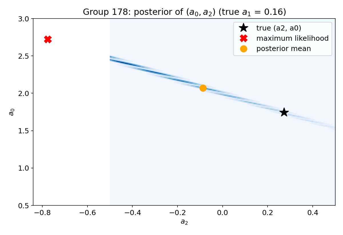
The posterior of (a2, a0) for one training group, shown as a thin dark diagonal band running from (a2 = -0.5, a0 = 2.5) to (0.5, 1.5) inside the parameter box. The true value lies on the band; the maximum-likelihood estimate lies outside the box at a2 = -0.78; the posterior mean sits in the middle of the band, much closer to the truth.

The full solution

For each group (solve_group in solution.py):

Run annealed, Sinkhorn-balanced EM from two starts (box centres, plus one random draw from the box), keep the higher likelihood.
Run the pairwise swap search until no swap improves the likelihood.
Using the final responsibilities as weights, replace the exponential, log and line parameters by their posterior means under the uniform box prior; canonicalise the sine ( $c_0 > 0$ , $c_2 \in (-\pi, \pi]$ ).

The core E-step is short:

for s in np.geomspace(1.0, SIGMA, iters):                  # annealing
    P = np.stack([f(k, th[k], x) for k in KS], 1)          # predictions of the 4 curves
    ll = -0.5 * ((y[:, None] - P) / s) ** 2 + np.log(px)   # px = uniform x-range densities
    R = np.exp(ll - ll.max(1, keepdims=True))
    for _ in range(30):                                     # Sinkhorn: 100 points per curve
        R /= R.sum(1, keepdims=True); R *= (n / 4) / R.sum(0, keepdims=True)
    th = {k: fit(k, x, y, R[:, j]) for j, k in enumerate(KS)}   # weighted M-step

A whole run (400 validation groups, then the 200 test groups) takes about 30 minutes on one CPU core and writes submission.csv in the sample-submission format.

Results

All RMSEs over the 11 parameters of the 400 training groups (true parameters known).

approach	RMSE
organisers' baseline: k-means + `curve_fit` (raw)	8687
same, clipped to the parameter box	1.009
constant: centre of every box	0.621
first EM: one start, unbounded fits, no balancing (20 groups)	93.8
EM, one start, bounded separable fits + Sinkhorn balancing (40 groups)	0.491
EM, four starts, maximum likelihood	0.155
same + posterior means	0.113
EM, two starts + swap search, maximum likelihood	0.097
same, clipped to the box	0.086
EM + swap search + posterior means (submitted)	0.0555

Per parameter, the final errors are $a_0$ : 0.112, $a_1$ : 0.011, $a_2$ : 0.135, $b_0$ : 0.022, $b_1$ : 0.038, $c_0$ : 0.018, $c_1$ : 0.003, $c_2$ : 0.023, $c_3$ : 0.013, $d_0$ : 0.006, $d_1$ : 0.014. The exponential's offset and amplitude carry most of the remaining error, and that error is mostly irreducible: it is the width of the posterior ridge, not a fitting failure.

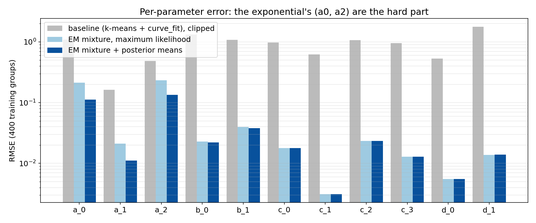
Per-parameter RMSE on a log scale for three methods: the clipped baseline (around 0.2 to 1.8), EM with maximum likelihood, and EM with posterior means. EM is 10 to 200 times better than the baseline on every parameter; posterior means mainly help a0, a1 and a2.

With the baseline at about 1.0 (clipped) or far above (raw), an RMSE of 0.056 is very close to the maximum $\frac{X_{\text{baseline}} - X}{X_{\text{baseline}} - X_{\text{best}}}$ can give: even a perfect predictor ( $X_{\text{best}} = 0$ ) would leave us above 94 % against the clipped baseline.

What to remember

When the labels of a mixture are missing, cluster with the model, not with distances. EM on a mixture of regressions assigns points to the curve that explains them.
EM finds local optima: help it. Annealing (start soft, end sharp), constraints you know to be true (balanced sizes, $x$ -ranges, parameter bounds) and explicit moves that escape known traps (swapping two components) matter more than more random restarts.
Separate linear and nonlinear parameters. Grid search over the one nonlinear parameter plus exact least squares is fast and never diverges.
Read the data for free priors: histograms revealed the $x$ -ranges, the training parameters revealed the box and the noise level.
Match the estimator to the metric: under squared error the optimal answer is the posterior mean; when a parameter is poorly identified, it beats maximum likelihood by a wide margin.

Full code (solution.py)

"""USAAIO 2026 Round 2 Day 2, Problem 5: mixed functions parameter regression.

Each group = 400 shuffled (x, y) points, 100 from each of
  exp: a0 exp(a1 x) + a2,  log: b0 ln x + b1,  sin: c0 sin(c1 x + c2) + c3,  lin: d0 x + d1
plus Gaussian noise.  Model: a 4-component MIXTURE OF REGRESSIONS fitted by EM
  - likelihood of a point under component k = U(x; domain_k) * N(y; f_k(x), sigma^2)
    (the x-domains, the parameter box and sigma = 0.12 are read off the training data)
  - deterministic annealing (sigma from 1.0 down to 0.12), 2 starts, then a
    pairwise "swap" search that escapes label-swap local optima
  - Sinkhorn-balanced responsibilities (each component owns exactly 100 points)
  - M-step: weighted least squares; the one nonlinear parameter (a1, c1) by grid
    search + bounded refinement
  - final estimate of exp / log / lin parameters = posterior MEAN under the uniform
    prior box (minimises expected squared error, which is what RMSE measures)
Validation: the 400 training groups (true parameters known).  Test: 200 groups.
Run:  python solution.py   (data in ./work: train.csv, train_params.csv, test.csv)
"""
import time
import numpy as np
import pandas as pd
from scipy.optimize import least_squares

D = "work/"
KS = ["exp", "log", "sin", "lin"]
DOM = {"exp": (0.5, 5.0), "log": (1.1, 10.0), "sin": (0.0, 4 * np.pi), "lin": (-3.0, 5.0)}
BOX = {"a_0": (0.5, 3), "a_1": (0.1, 0.8), "a_2": (-0.5, 0.5), "b_0": (0.5, 3), "b_1": (-1, 1),
       "c_0": (1, 3), "c_1": (0.5, 2), "c_2": (-1, 1), "c_3": (0, 2), "d_0": (0.3, 1.5), "d_1": (-2, 2)}
PNAMES = list(BOX)
LB = {"exp": [0.3, 0.05, -0.8], "sin": [0.7, 0.4, -10, -0.3]}      # loose bounds for the fits
UB = {"exp": [3.5, 0.9, 0.8], "sin": [3.5, 2.2, 10, 2.3]}
SIGMA = 0.12


def f(k, th, x):
    with np.errstate(all="ignore"):
        if k == "exp": return th[0] * np.exp(np.clip(th[1] * x, -50, 50)) + th[2]
        if k == "log": return th[0] * np.log(np.where(x > 0, x, np.nan)) + th[1]
        if k == "sin": return th[0] * np.sin(th[1] * x + th[2]) + th[3]
        return th[0] * x + th[1]


def wls(A, y, w):
    Aw = A * w[:, None]
    return np.linalg.solve(A.T @ Aw + 1e-9 * np.eye(A.shape[1]), Aw.T @ y)


def fit(k, x, y, w):
    """Weighted fit of one family (M-step)."""
    m = w > 1e-6
    x, y, w = x[m], y[m], w[m]
    if k == "lin": return wls(np.c_[x, np.ones_like(x)], y, w)
    if k == "log": return wls(np.c_[np.log(x), np.ones_like(x)], y, w)
    best = None
    if k == "exp":            # given a1 the model is linear in (a0, a2)
        for a1 in np.linspace(0.08, 0.85, 40):
            A = np.c_[np.exp(a1 * x), np.ones_like(x)]; c = wls(A, y, w)
            r = np.sum(w * (A @ c - y) ** 2)
            if best is None or r < best[0]: best = (r, np.array([c[0], a1, c[1]]))
    else:                     # given c1: c0 sin(c1x+c2) = s sin(c1x) + co cos(c1x)
        for c1 in np.linspace(0.45, 2.05, 81):
            A = np.c_[np.sin(c1 * x), np.cos(c1 * x), np.ones_like(x)]; c = wls(A, y, w)
            r = np.sum(w * (A @ c - y) ** 2)
            if best is None or r < best[0]:
                best = (r, np.array([np.hypot(c[0], c[1]), c1, np.arctan2(c[1], c[0]), c[2]]))
    lo, hi = np.array(LB[k]), np.array(UB[k])
    th = np.clip(best[1], lo + 1e-9, hi - 1e-9)
    sw = np.sqrt(w)
    return least_squares(lambda t: sw * (f(k, t, x) - y), th, bounds=(lo, hi)).x


def em(x, y, init, iters=40, s0=1.0):
    n = len(x)
    px = np.stack([((x >= a) & (x <= b)) / (b - a) for a, b in (DOM[k] for k in KS)], 1)
    th = dict(init)
    for s in np.geomspace(s0, SIGMA, iters):          # deterministic annealing
        P = np.stack([f(k, th[k], x) for k in KS], 1)
        ll = -0.5 * ((y[:, None] - P) / s) ** 2
        ll = np.where(np.isfinite(ll) & (px > 0), ll + np.log(px + 1e-300), -np.inf)
        R = np.exp(ll - ll.max(1, keepdims=True))
        for _ in range(30):                             # Sinkhorn: rows -> 1, columns -> n/4
            R /= R.sum(1, keepdims=True) + 1e-300
            R *= (n / 4) / (R.sum(0, keepdims=True) + 1e-300)
        R /= R.sum(1, keepdims=True)
        for j, k in enumerate(KS):
            try: th[k] = fit(k, x, y, R[:, j])
            except Exception: pass
    P = np.nan_to_num(np.stack([f(k, th[k], x) for k in KS], 1), nan=1e9)
    dens = px * np.exp(-0.5 * ((y[:, None] - P) / SIGMA) ** 2)
    return th, np.log(dens.sum(1) + 1e-300).sum(), R


def random_init(rng):
    u = lambda k: rng.uniform(*BOX[k])
    return {"exp": np.array([u("a_0"), u("a_1"), u("a_2")]), "log": np.array([u("b_0"), u("b_1")]),
            "sin": np.array([u("c_0"), u("c_1"), u("c_2"), u("c_3")]), "lin": np.array([u("d_0"), u("d_1")])}


CENTER = {"exp": np.array([1.75, 0.45, 0.0]), "log": np.array([1.75, 0.0]),
          "sin": np.array([2.0, 1.25, 0.0, 1.0]), "lin": np.array([0.9, 0.0])}


def swap_search(x, y, best):
    """Escape label-swap local optima: for every pair of families, refit each one on the
    points the other currently owns, re-run a short cool EM, keep it if the likelihood rises."""
    improved = True
    while improved:
        improved = False
        th, L, R = best
        for i in range(4):
            for j in range(i + 1, 4):
                ki, kj = KS[i], KS[j]
                new = {k: v.copy() for k, v in th.items()}
                try:
                    di, dj = DOM[ki], DOM[kj]
                    wi = R[:, j] * ((x >= di[0]) & (x <= di[1]))
                    wj = R[:, i] * ((x >= dj[0]) & (x <= dj[1]))
                    new[ki], new[kj] = fit(ki, x, y, wi), fit(kj, x, y, wj)
                except Exception:
                    continue
                res = em(x, y, new, iters=20, s0=0.3)
                if res[1] > best[1] + 1e-6:
                    best, improved = res, True
    return best


def canon_sin(th):
    c0, c1, c2, c3 = th
    if c0 < 0: c0, c2 = -c0, c2 + np.pi
    return np.array([c0, c1, (c2 + np.pi) % (2 * np.pi) - np.pi, c3])


def post_mean_2(phi, y, w, b0, b1, n=121):
    """Posterior mean of (p0, p1) in y = p0 phi + p1 + N(0, sigma^2), uniform prior on a box."""
    g0 = np.linspace(*b0, n)[:, None]; g1 = np.linspace(*b1, n)[None, :]
    S = [w.sum(), (w * phi).sum(), (w * phi * phi).sum(), (w * y).sum(), (w * y * phi).sum(), (w * y * y).sum()]
    rss = S[5] - 2 * g0 * S[4] - 2 * g1 * S[3] + g0 ** 2 * S[2] + 2 * g0 * g1 * S[1] + g1 ** 2 * S[0]
    P = np.exp(-(rss - rss.min()) / (2 * SIGMA ** 2)); P /= P.sum()
    return np.array([(P * g0).sum(), (P * g1).sum()])


def post_mean_exp(x, y, w):
    g1 = np.linspace(*BOX["a_1"], 141)
    g0 = np.linspace(*BOX["a_0"], 101)[:, None]; g2 = np.linspace(*BOX["a_2"], 81)[None, :]
    Sw, Sy, Syy = w.sum(), (w * y).sum(), (w * y * y).sum()
    LP = np.empty((len(g1), g0.size, g2.size))
    for i, a1 in enumerate(g1):
        e = np.exp(a1 * x); Se, See, Sye = (w * e).sum(), (w * e * e).sum(), (w * y * e).sum()
        LP[i] = -(Syy - 2 * g0 * Sye - 2 * g2 * Sy + g0 ** 2 * See + 2 * g0 * g2 * Se + g2 ** 2 * Sw) / (2 * SIGMA ** 2)
    P = np.exp(LP - LP.max()); P /= P.sum()
    return np.array([(P.sum((0, 2)) * g0[:, 0]).sum(), (P.sum((1, 2)) * g1).sum(), (P.sum((0, 1)) * g2[0]).sum()])


def solve_group(x, y, n_starts=2, seed=0):
    rng = np.random.default_rng(seed)
    best = None
    for s in range(n_starts):
        res = em(x, y, CENTER if s == 0 else random_init(rng))
        if best is None or res[1] > best[1]: best = res
    best = swap_search(x, y, best)
    th, _, R = best
    mle = np.r_[th["exp"], th["log"], canon_sin(th["sin"]), th["lin"]]
    m0, m1, m3 = R[:, 0] > 1e-3, (R[:, 1] > 1e-3) & (x > 0), R[:, 3] > 1e-3
    bayes = np.r_[post_mean_exp(x[m0], y[m0], R[m0, 0]),
                  post_mean_2(np.log(x[m1]), y[m1], R[m1, 1], BOX["b_0"], BOX["b_1"]),
                  canon_sin(th["sin"]),
                  post_mean_2(x[m3], y[m3], R[m3, 3], BOX["d_0"], BOX["d_1"])]
    return mle, bayes, R.argmax(1)


def job(args):
    x, y = args
    return solve_group(x, y)


def run(df):
    groups = sorted(df.group_id.unique())
    data = [(df.x.values[df.group_id.values == g], df.y.values[df.group_id.values == g]) for g in groups]
    out = [job(d) for d in data]          # single process (shared machine)
    return groups, np.array([o[0] for o in out]), np.array([o[1] for o in out])


def baseline(x, y):
    """The organisers' baseline: k-means (k=4) on (x, y), fit every family on every cluster
    with curve_fit, keep for each family the cluster it fits best."""
    from scipy.optimize import curve_fit
    from sklearn.cluster import KMeans
    fams = {"exp": (lambda x, a, b, c: a * np.exp(b * x) + c, [1.75, 0.45, 0.0]),
            "log": (lambda x, a, b: a * np.log(np.abs(x) + 1e-9) + b, [1.75, 0.0]),
            "sin": (lambda x, a, b, c, d: a * np.sin(b * x + c) + d, [2.0, 1.25, 0.0, 1.0]),
            "lin": (lambda x, a, b: a * x + b, [0.9, 0.0])}
    lab = KMeans(4, n_init=10, random_state=0).fit_predict(
        np.c_[(x - x.mean()) / x.std(), (y - y.mean()) / y.std()])
    out = []
    for fn, p0 in fams.values():
        best = (np.inf, p0)
        for c in range(4):
            m = lab == c
            try:
                th, _ = curve_fit(fn, x[m], y[m], p0=p0, maxfev=5000)
                mse = np.mean((fn(x[m], *th) - y[m]) ** 2)
                if mse < best[0]: best = (mse, th)
            except Exception:
                pass
        out += list(best[1])
    return np.array(out)


def rmse(pred, true):
    return np.sqrt(((pred - true) ** 2).mean())


if __name__ == "__main__":
    t0 = time.time()
    train = pd.read_csv(D + "train.csv")
    params = pd.read_csv(D + "train_params.csv").set_index("group_id")
    test = pd.read_csv(D + "test.csv")
    lo = np.array([BOX[k][0] for k in PNAMES]); hi = np.array([BOX[k][1] for k in PNAMES])

    g, mle, bayes = run(train)
    true = params.loc[g, PNAMES].values
    centre = np.tile((lo + hi) / 2, (len(g), 1))
    print("validation on 400 training groups (RMSE over all 11 x 400 parameters)")
    print("  constant = centre of the box   %.4f" % rmse(centre, true))
    if "--baseline" in __import__("sys").argv:
        base = np.array([baseline(train.x.values[train.group_id.values == k],
                                  train.y.values[train.group_id.values == k]) for k in g])
        print("  baseline (raw / clipped)       %.1f / %.4f" % (rmse(base, true), rmse(np.clip(base, lo, hi), true)))
    print("  EM, maximum likelihood         %.4f" % rmse(mle, true))
    print("  EM, ML clipped to the box      %.4f" % rmse(np.clip(mle, lo, hi), true))
    print("  EM + posterior means           %.4f" % rmse(bayes, true))
    per = pd.DataFrame({"ML": np.sqrt(((mle - true) ** 2).mean(0)),
                        "Bayes": np.sqrt(((bayes - true) ** 2).mean(0))}, index=PNAMES)
    print(per.round(4).T)
    np.save(D + "val_pred.npy", np.stack([mle, bayes]))

    gt, _, bt = run(test)
    sub = pd.DataFrame(bt, columns=PNAMES); sub.insert(0, "group_id", gt)
    sub.to_csv(D + "submission.csv", index=False)
    print("wrote", D + "submission.csv", sub.shape, "in %.1f min" % ((time.time() - t0) / 60))