← Back to the problem

USA USAAIO 2026 Β· Correction by IOAI Training

Linear Attention Is All You Need

This page gives the full approach. Read it once you have searched.

Metric
macro F1 (Part 1.4) + written parts
Evaluated on
official test (UCR FordA test labels are public)
Our score
0.944 macro F1 on test; derivations done

We solved the problem ourselves: downloaded the data, ran the experiments and measured the score below. The statement and data belong to their organisers.

The problem in brief

This 90-point problem from the 2026 USA AI Olympiad Round 2 (Day 1, Problem 1) walks from theory to practice. First it asks why standard attention costs O(T2)O(T^2) and how a feature map Ο•\phi with exp⁑(q⊀k/d)=Ο•(q)βŠ€Ο•(k)\exp(q^\top k/\sqrt d) = \phi(q)^\top\phi(k) makes attention linear in TT. Next it covers why an exact Ο•\phi would need infinitely many features, and how to build one from a truncated Taylor series. Then it adds relative positional encodings rjβˆ’ir_{j-i} to the attention scores and asks you to fit them into the linear-attention framework. Finally you must implement the module in PyTorch, with Ο•(x)=1+ELU(x)\phi(x) = 1 + \text{ELU}(x), build an encoder-only transformer from it, and classify the FordA engine-noise time series (500 samples each, 2 classes), with no other positional encoding allowed.

FordA is a public UCR archive dataset. The competition's test.csv matches the official UCR test file row for row, so we can score our final model on the real test set: the labels were used once, at the very end, and never for any choice.

How you are scored

Parts 1.1 to 1.3 are marked on correct reasoning and code. Part 1.4 (20 points) is marked on test macro F1, relative to the best submission: 100 Xβˆ’0.5Xbestβˆ’0.5100\,\frac{X - 0.5}{X_\text{best} - 0.5}, since random guessing gives 0.5. The best contestant's score is not published.

Part 1.1: linear attention

1.1.1 Complexity. QK⊀QK^\top is a TΓ—TT\times T matrix whose entries each need a dot product of length dd: O(T2d)O(T^2 d). The row-wise softmax costs O(T2)O(T^2), and multiplying the TΓ—TT\times T weights by V∈RTΓ—dV \in \mathbb{R}^{T\times d} costs O(T2d)O(T^2 d) again. Total: O(T2d)O(T^2 d) time, plus O(T2)O(T^2) memory for the attention matrix. Doubling the sequence length quadruples the cost.

1.1.2 Output with a feature map. Softmax attention is a weighted average,

ot=βˆ‘jexp⁑(qt⊀kj/d) vjβˆ‘jexp⁑(qt⊀kj/d)=βˆ‘jΟ•(qt)βŠ€Ο•(kj) vjβˆ‘jΟ•(qt)βŠ€Ο•(kj).o_t = \frac{\sum_j \exp(q_t^\top k_j/\sqrt d)\, v_j}{\sum_j \exp(q_t^\top k_j/\sqrt d)} = \frac{\sum_j \phi(q_t)^\top\phi(k_j)\, v_j}{\sum_j \phi(q_t)^\top\phi(k_j)} .

Since Ο•(qt)βŠ€Ο•(kj)\phi(q_t)^\top\phi(k_j) is a scalar, (Ο•(qt)βŠ€Ο•(kj)) vj=vj ϕ(kj)βŠ€Ο•(qt)\big(\phi(q_t)^\top\phi(k_j)\big)\, v_j = v_j\,\phi(k_j)^\top\phi(q_t), and Ο•(qt)\phi(q_t) can be pulled out of both sums:

ot=(βˆ‘jvj ϕ(kj)⊀) ϕ(qt)Ο•(qt)βŠ€βˆ‘jΟ•(kj).o_t = \frac{\Big(\sum_j v_j\,\phi(k_j)^\top\Big)\,\phi(q_t)}{\phi(q_t)^\top \sum_j \phi(k_j)} .

The two sums no longer depend on tt: they are computed once and shared by every query.

1.1.3 Matrix form. Stacking the rows, βˆ‘jΟ•(kj)vj⊀=Ο•(K)⊀V∈Rβ„“Γ—d\sum_j \phi(k_j) v_j^\top = \phi(K)^\top V \in \mathbb{R}^{\ell\times d} and βˆ‘jΟ•(kj)=Ο•(K)⊀1T\sum_j \phi(k_j) = \phi(K)^\top \mathbf 1_T. So

O=diag⁑ ⁣(Ο•(Q) ϕ(K)⊀1T)βˆ’1Β Ο•(Q) (Ο•(K)⊀V).O = \operatorname{diag}\!\big(\phi(Q)\,\phi(K)^\top \mathbf 1_T\big)^{-1}\ \phi(Q)\,\big(\phi(K)^\top V\big).

Each row of the numerator is divided by the corresponding entry of Ο•(Q)(Ο•(K)⊀1T)\phi(Q)\big(\phi(K)^\top\mathbf 1_T\big). The brackets matter: computing Ο•(K)⊀V\phi(K)^\top V first is what avoids the TΓ—TT\times T matrix.

1.1.4 Complexity with β„“\ell features. Ο•(K)⊀V\phi(K)^\top V: O(Tβ„“d)O(T\ell d). Ο•(Q)\phi(Q) times that β„“Γ—d\ell\times d matrix: O(Tβ„“d)O(T\ell d). The denominator: O(Tβ„“)O(T\ell) for Ο•(K)⊀1\phi(K)^\top\mathbf 1 and O(Tβ„“)O(T\ell) for the product with Ο•(Q)\phi(Q). The normalisation: O(Td)O(Td). Total: O(Tβ„“d)O(T\ell d), linear in TT, with memory O(β„“d+T(β„“+d))O(\ell d + T(\ell + d)).

1.1.5 Why β„“=∞\ell = \infty. With x=q⊀k/dx = q^\top k/\sqrt d, the series exp⁑(x)=βˆ‘rxr/r!\exp(x) = \sum_r x^r/r! contains every power of the dot product. Each power is itself an inner product of tensor powers: (q⊀k)r=⟨qβŠ—r,kβŠ—r⟩(q^\top k)^r = \langle q^{\otimes r}, k^{\otimes r}\rangle, with drd^r coordinates. So

exp⁑(q⊀kd)=βˆ‘r=0∞⟨qβŠ—rr! dr/4,kβŠ—rr! dr/4⟩,\exp\Big(\frac{q^\top k}{\sqrt d}\Big) = \sum_{r=0}^{\infty} \Big\langle \frac{q^{\otimes r}}{\sqrt{r!}\,d^{r/4}}, \frac{k^{\otimes r}}{\sqrt{r!}\,d^{r/4}} \Big\rangle,

and the natural feature map has βˆ‘rdr=∞\sum_r d^r = \infty coordinates. No finite β„“\ell can work either. If Ο•\phi had β„“\ell features, then for any TT vectors x1,…,xTx_1,\dots,x_T the matrix Mij=exp⁑(xi⊀xj/d)M_{ij} = \exp(x_i^\top x_j/\sqrt d) would equal Ο•(X)Ο•(X)⊀\phi(X)\phi(X)^\top and have rank at most β„“\ell. But the exponential kernel is strictly positive definite: for distinct points this matrix is invertible, so its rank is TT. Taking T>β„“T > \ell points gives a contradiction, so the representation requires β„“=∞\ell = \infty.

1.1.6 A finite map from the truncated series. With x=q⊀k/dx = q^\top k/\sqrt d, approximate exp⁑(x)β‰ˆ1+x+x2/2\exp(x) \approx 1 + x + x^2/2. Using (q⊀k)2=βˆ‘a,bqaqb kakb=⟨vec⁑(qq⊀),vec⁑(kk⊀)⟩(q^\top k)^2 = \sum_{a,b} q_a q_b\, k_a k_b = \langle \operatorname{vec}(qq^\top), \operatorname{vec}(kk^\top)\rangle, define

Ο•(z)=(1,Β zd1/4,Β vec⁑(zz⊀)2 d)∈R1+d+d2.\phi(z) = \Big(1,\ \frac{z}{d^{1/4}},\ \frac{\operatorname{vec}(z z^\top)}{\sqrt 2\,\sqrt d}\Big) \in \mathbb{R}^{1 + d + d^2}.

Then Ο•(q)βŠ€Ο•(k)=1+q⊀kd+(q⊀k)22d\phi(q)^\top\phi(k) = 1 + \frac{q^\top k}{\sqrt d} + \frac{(q^\top k)^2}{2d}, exactly the truncated series. So β„“=1+d+d2\ell = 1 + d + d^2. Since zz⊀zz^\top is symmetric, keeping only a≀ba \le b (with weight 2\sqrt 2 on off-diagonal terms) reduces this to β„“=1+d+d(d+1)2\ell = 1 + d + \frac{d(d+1)}{2}. A bonus: 1+x+x2/2=12((x+1)2+1)>01 + x + x^2/2 = \frac{1}{2}\big((x+1)^2 + 1\big) > 0 for every xx, so the approximate attention weights stay positive and the normaliser never vanishes.

Part 1.2: relative positional encoding

1.2.1 When it is the better choice. It is better when what matters is how far apart two events are, not where they sit in the window: stationary signals, periodic patterns, and windows cut at arbitrary moments. FordA is exactly this case. A 500-sample snippet of engine noise starts at an arbitrary time, so "position 37" means nothing, while "an event 12 samples after another" may well be the fault signature. Relative encodings make the attention pattern (approximately) translation-equivariant, share parameters across all positions with the same lag, and generalise better to positions or lengths unseen in training. Absolute encodings are better when absolute position carries meaning (the first token of a sentence, a fixed time of day).

1.2.2 Range of jβˆ’ij - i. With i,j∈{0,…,Tβˆ’1}i, j \in \{0,\dots,T-1\}, the lag jβˆ’ij - i ranges from 0βˆ’(Tβˆ’1)=βˆ’(Tβˆ’1)0 - (T-1) = -(T-1) to (Tβˆ’1)βˆ’0=Tβˆ’1(T-1) - 0 = T-1, so there are 2Tβˆ’12T - 1 possible values, and therefore 2Tβˆ’12T-1 vectors rmr_m to learn (per head).

1.2.3 Initial scale Ο„2\tau^2. The score is qi⊀kj+qi⊀rjβˆ’iq_i^\top k_j + q_i^\top r_{j-i}. With independent zero-mean components, Var⁑(qi⊀kj)=d σq2Οƒ2\operatorname{Var}(q_i^\top k_j) = d\,\sigma_q^2\sigma^2 and Var⁑(qi⊀rjβˆ’i)=d σq2Ο„2\operatorname{Var}(q_i^\top r_{j-i}) = d\,\sigma_q^2\tau^2. To let neither the content term nor the positional term dominate at initialisation, make them equal: Ο„2=Οƒ2\tau^2 = \sigma^2. A much smaller Ο„\tau means position is ignored at first, and the gradient that would teach it is tiny. A much larger Ο„\tau means the content is drowned out. (The total score variance then doubles. If you want to keep it unchanged, scale kj+rjβˆ’ik_j + r_{j-i} by 1/21/\sqrt 2.) In the code, Οƒ2\sigma^2 is the variance of the key projections at initialisation, about 1/31/3 with PyTorch's default nn.Linear initialisation and unit-variance inputs.

1.2.4 Relative positions inside linear attention. Plugging kj+rjβˆ’ik_j + r_{j-i} into a feature map does not factorise, because the "key" would then depend on ii. We instead use the sum of two positive kernels, one for content and one for position:

sim⁑(i,j)=Ο•(qi)βŠ€Ο•(kj)+Ο•(qi)βŠ€Ο•(rjβˆ’i),\operatorname{sim}(i,j) = \phi(q_i)^\top\phi(k_j) + \phi(q_i)^\top\phi(r_{j-i}), oi=Ο•(qi)⊀(Ο•(K)⊀V+Si)Ο•(qi)⊀(Ο•(K)⊀1+si),Si=βˆ‘jΟ•(rjβˆ’i) vj⊀,si=βˆ‘jΟ•(rjβˆ’i).o_i = \frac{\phi(q_i)^\top\big(\phi(K)^\top V + S_i\big)}{\phi(q_i)^\top\big(\phi(K)^\top\mathbf 1 + s_i\big)}, \qquad S_i = \sum_j \phi(r_{j-i})\,v_j^\top, \qquad s_i = \sum_j \phi(r_{j-i}).

Both kernels are positive, so the weights stay positive and the normaliser never vanishes. The content part costs O(Tβ„“d)O(T\ell d) as before. SiS_i is a cross-correlation along time between the sequence of lags Ο•(rm)\phi(r_m) and the values vjv_j, so the FFT computes it for all ii in O(β„“d Tlog⁑T)O(\ell d\, T\log T). And sis_i is a sum over a sliding window of lags, which prefix sums give in O(Tβ„“)O(T\ell). Everything stays (almost) linear in TT, and no TΓ—TT\times T matrix is ever formed. This is the Toeplitz structure behind relative-position linear transformers. A simpler alternative is a learned scalar bias bjβˆ’ib_{j-i} multiplying the weights, but the version above follows the statement's vector form rjβˆ’ir_{j-i}.

Part 1.3: implementation

1.3.1 Number of parameters (no biases). The query, key and value projections each map dmodeld_\text{model} to Hβ‹…dH\cdot d, and the output projection maps Hβ‹…dH\cdot d back to dmodeld_\text{model}. Each head has 2Tβˆ’12T-1 relative vectors of length dd:

#params=3 dmodelHd+Hd dmodel+(2Tβˆ’1)Hd=4 dmodelHd+(2Tβˆ’1)Hd.\#\text{params} = 3\,d_\text{model}Hd + Hd\,d_\text{model} + (2T-1)Hd = 4\,d_\text{model}Hd + (2T-1)Hd .

For dmodel=32d_\text{model}=32, T=50T=50, H=4H=4, d=8d=8 this gives 4096+3168=72644096 + 3168 = 7264, which matches PyTorch's count.

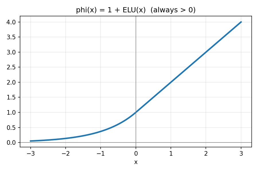
1.3.2 Plots. ELU(x)\text{ELU}(x) is the identity for xβ‰₯0x \ge 0 and exβˆ’1∈(βˆ’1,0)e^x - 1 \in (-1, 0) for x<0x<0, so Ο•(x)=1+ELU(x)\phi(x) = 1 + \text{ELU}(x) is strictly positive, smooth at 0 (slope 1 on both sides) and grows linearly. Strict positivity is what we need: the similarities must be positive for the weights to form an average.
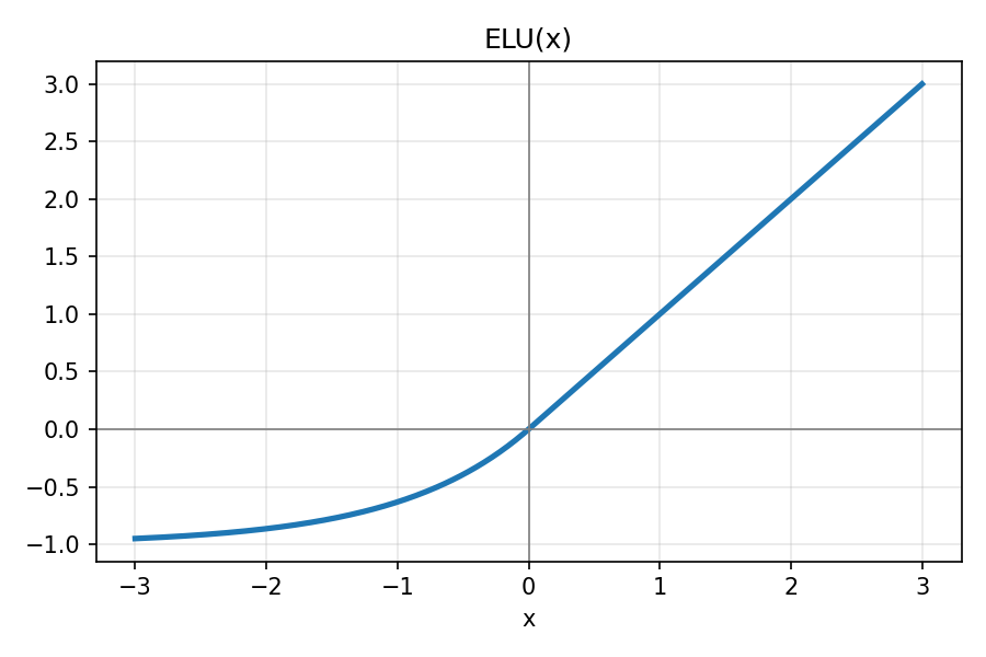
ELU

phi = 1 + ELU

1.3.3 The module. The core of MyLinearAttentionRelativePos.forward (the full class is in solution.py):

q, k = phi(W_q(x)), phi(W_k(x))                 # (B, H, T, d) after reshaping into heads
v, pr = W_v(x), phi(self.r)                     # pr: (H, 2T-1, d), one vector per lag
kv  = einsum('bhtl,bhtc->bhlc', k, v)           # phi(K)^T V
num = einsum('bhtl,bhlc->bhtc', q, kv)
den = einsum('bhtl,bhl->bht', q, k.sum(2))
S = irfft(rfft(pr.flip(1), n=4T)[..., None] * rfft(v, n=4T)[..., None, :])[:, :, T-1:2T-1]
num += einsum('bhtl,bhtlc->bhtc', q, S)         # positional part via FFT correlation
den += einsum('bhtl,htl->bht', q, window_sums(pr))
out = W_o((num / den).merge_heads())

We checked it against a direct O(T2)O(T^2) computation of the same similarity: the outputs agree to 10βˆ’1610^{-16} in double precision. The relative vectors are initialised with standard deviation equal to that of the keys, following 1.2.3.

Part 1.4: a transformer for FordA

The data. 3 601 training and 1 320 test series of 500 engine-noise samples, each already normalised to zero mean and unit variance, with two balanced classes (the symptom is present or absent). Two quick baselines tell us what kind of signal this is. Logistic regression on the raw samples is at chance (macro F1 0.51), because the series are not aligned in time. On the log magnitude of the Fourier spectrum it reaches 0.91. The class information is mostly in which frequencies and patterns appear, not where. That is exactly the setting in which relative positional encoding makes sense (Part 1.2.1).

The model (FordATransformer in solution.py):

  1. Cut the series into T=50T = 50 patches of 10 samples and map each patch to dmodel=64d_\text{model} = 64 with one linear layer. Following the rules, no positional encoding is added at the input: position enters only through the relative terms rjβˆ’ir_{j-i} inside attention.
  2. Three pre-norm encoder blocks: LayerNorm, then our linear attention (H=4H = 4 heads, d=16d = 16), plus a residual connection; then LayerNorm, an MLP 64β†’128β†’6464 \to 128 \to 64 with GELU, plus a residual connection. Dropout is 0.1.
  3. Average the 50 tokens, apply LayerNorm, then a linear layer to 2 logits. About 120 k parameters.
  4. Training: AdamW (weight decay 0.05), one-cycle learning rate peaking at 10βˆ’310^{-3}, batches of 64, label smoothing 0.05, gradient clipping at 1, 80 epochs. Augmentation: a random circular time shift and a random amplitude scale (0.8 to 1.2). The shift encodes the same translation invariance as the relative encoding: a fault pattern is the same fault wherever it appears in the window.

We tuned on a random 80/20 split of the training set, then retrained on all 3 601 series and predicted the test set once. FordA is a public UCR dataset, and the competition's test.csv is identical, row for row, to the UCR test file. That lets us report the true test score.

Results

approachdatamacro F1
random guessing0.50
logistic regression on raw samplesvalidation split0.508
logistic regression on log-spectrumvalidation split0.912
transformer, 40 epochs, no augmentationvalidation split0.919
transformer, 40 epochs, shift + scale augmentationvalidation split0.932
transformer, 80 epochs, augmentation, patches of 5 (T=100T = 100)validation split0.908
transformer, 80 epochs, augmentation, patches of 10 (T=50T = 50)validation split0.942
final: same model trained on all training dataofficial test (1 320)0.944 (accuracy 94.4 %)

The competition mark is relative to the best submission, which is not published, so there is no target to compare with. For context, the description file shipped with the UCR archive says the winning entry of the original 2008 competition reported 100 % test accuracy on FordA, so there is still room above our 94.4 %. We trained on Apple MPS (about 10 minutes per run), not on the L4 GPU the rules require for the notebook; nothing in the code depends on the device.

What to remember

  • Softmax attention costs O(T2d)O(T^2 d) because of the TΓ—TT\times T matrix. A kernel feature map Ο•\phi lets you compute Ο•(K)⊀V\phi(K)^\top V first, which brings the cost down to O(Tβ„“d)O(T\ell d).
  • The exact exponential kernel needs infinitely many features (its Gram matrices have full rank). Truncated Taylor maps (β„“=1+d+d2\ell = 1 + d + d^2) or positive maps like 1+ELU1 + \text{ELU} are practical substitutes.
  • Relative positions fit into linear attention as a second positive kernel. Their contribution is a correlation over lags, which the FFT computes in O(Tlog⁑T)O(T\log T).
  • Initialise new score terms at the same scale as the existing ones (Ο„2=Οƒ2\tau^2 = \sigma^2), so neither dominates at the start.
  • Match the inductive bias to the data. FordA is shift-invariant (the raw-sample model is at chance while the spectrum model works), so relative encoding plus shift augmentation is the right recipe.
  • Test any fast implementation against a slow, obviously correct one. Ours matched the O(T2)O(T^2) version to 10βˆ’1610^{-16}.
Full code (solution.py)
"""USAAIO 2026 Round 2, Problem 1: linear attention with relative positional encoding, and an
encoder-only transformer built on it for FordA (engine-noise series of length 500, 2 classes).

  python3 solution.py   (run from the folder holding work/train.csv, work/test.csv,
                         work/sample_submission.csv and the public UCR file work/FordA_TEST.txt)
Steps: unit test of the fast attention against an explicit O(T^2) computation; ELU / phi plots;
baselines and the transformer on an 80/20 split of train.csv; final model on all of train.csv,
scored once on the official test labels (FordA is a public UCR dataset) and written to CSV.
"""
import warnings; warnings.filterwarnings('ignore')
import numpy as np, pandas as pd, torch, torch.nn as nn, torch.nn.functional as F, time, sys
import matplotlib; matplotlib.use('Agg'); import matplotlib.pyplot as plt
from sklearn.linear_model import LogisticRegression


class MyLinearAttentionRelativePos(nn.Module):
    """Multi-head linear self-attention with learnable relative positional encodings.

    similarity(i, j) = phi(q_i).phi(k_j) + phi(q_i).phi(r_{j-i}),   phi(x) = 1 + ELU(x)
    o_i = sum_j sim(i,j) v_j / sum_j sim(i,j)
    The content term is computed in O(T l d) with the usual (phi(K)^T V) trick; the positional
    term is a cross-correlation over the lag j-i, computed with FFTs in O(l d T log T).
    """

    def __init__(self, d_model, T, H, d):
        super().__init__()
        self.T, self.H, self.d = T, H, d
        self.W_q = nn.Linear(d_model, H * d, bias=False)
        self.W_k = nn.Linear(d_model, H * d, bias=False)
        self.W_v = nn.Linear(d_model, H * d, bias=False)
        self.W_o = nn.Linear(H * d, d_model, bias=False)
        # r[h, m] for lag m - (T-1) in {-(T-1), ..., T-1}; std 1 matches the keys' scale (Part 1.2.3)
        self.r = nn.Parameter(torch.randn(H, 2 * T - 1, d) * self.W_k.weight.std().item() * d_model ** 0.5)
        self.elu = nn.ELU()

    def phi(self, x):
        return 1 + self.elu(x)

    def forward(self, x):                                   # x: (B, T, d_model)
        B, T, _ = x.shape
        H, d = self.H, self.d
        q = self.phi(self.W_q(x).view(B, T, H, d).transpose(1, 2))      # (B, H, T, d)
        k = self.phi(self.W_k(x).view(B, T, H, d).transpose(1, 2))
        v = self.W_v(x).view(B, T, H, d).transpose(1, 2)
        pr = self.phi(self.r)                                          # (H, 2T-1, d)

        # content part: phi(Q) (phi(K)^T V) and phi(Q) (phi(K)^T 1)
        kv = torch.einsum('bhtl,bhtc->bhlc', k, v)                     # (B, H, l, d)
        num = torch.einsum('bhtl,bhlc->bhtc', q, kv)
        den = torch.einsum('bhtl,bhl->bht', q, k.sum(2))

        # positional part: S_i = sum_j phi(r_{j-i}) v_j^T, a correlation along time -> FFT
        n = 4 * T                                                      # >= 3T-2: no wrap-around
        Rf = torch.fft.rfft(pr.flip(1), n=n, dim=1)                    # (H, n/2+1, l)
        Vf = torch.fft.rfft(v, n=n, dim=2)                             # (B, H, n/2+1, d)
        S = torch.fft.irfft(Rf[None, :, :, :, None] * Vf[:, :, :, None, :], n=n, dim=2)
        S = S[:, :, T - 1:2 * T - 1]                                   # (B, H, T, l, d), row i
        num = num + torch.einsum('bhtl,bhtlc->bhtc', q, S)
        csum = torch.cumsum(F.pad(pr, (0, 0, 1, 0)), dim=1)            # prefix sums over lags
        rsum = csum[:, 2 * T - 1 - torch.arange(T)] - csum[:, T - 1 - torch.arange(T)]  # (H, T, l)
        den = den + torch.einsum('bhtl,htl->bht', q, rsum)

        o = (num / den[..., None]).transpose(1, 2).reshape(B, T, H * d)
        return self.W_o(o)


def reference(m, x):
    """Same similarity computed explicitly in O(T^2): used to test the fast version."""
    B, T, _ = x.shape; H, d = m.H, m.d
    q = m.phi(m.W_q(x).view(B, T, H, d).transpose(1, 2)); k = m.phi(m.W_k(x).view(B, T, H, d).transpose(1, 2))
    v = m.W_v(x).view(B, T, H, d).transpose(1, 2)
    lag = torch.arange(T)[None, :] - torch.arange(T)[:, None] + T - 1          # (i, j) -> j - i + T - 1
    R = m.phi(m.r)[:, lag]                                                    # (H, T, T, d)
    sim = torch.einsum('bhil,bhjl->bhij', q, k) + torch.einsum('bhil,hijl->bhij', q, R)
    o = torch.einsum('bhij,bhjc->bhic', sim / sim.sum(-1, keepdim=True), v)
    return m.W_o(o.transpose(1, 2).reshape(B, T, H * d))


from sklearn.metrics import f1_score
torch.set_num_threads(2)
PATCH = 10
DEV = 'mps' if torch.backends.mps.is_available() else 'cpu'


class Block(nn.Module):
    def __init__(s, dm, T, H, d, hidden, p):
        super().__init__()
        s.n1, s.att, s.n2 = nn.LayerNorm(dm), MyLinearAttentionRelativePos(dm, T, H, d), nn.LayerNorm(dm)
        s.mlp = nn.Sequential(nn.Linear(dm, hidden), nn.GELU(), nn.Dropout(p), nn.Linear(hidden, dm))
        s.drop = nn.Dropout(p)
    def forward(s, x):
        x = x + s.drop(s.att(s.n1(x)))                     # pre-norm residual blocks
        return x + s.drop(s.mlp(s.n2(x)))


class FordATransformer(nn.Module):
    """Series of length 500 -> 50 patches of 10 samples (a linear 'patch embedding', no positional
    encoding) -> encoder blocks with relative-position linear attention -> mean pool -> 2 logits."""
    def __init__(s, L=500, patch=PATCH, dm=64, H=4, d=16, depth=3, hidden=128, p=0.1):
        super().__init__()
        s.patch, s.T = patch, L // patch
        s.embed = nn.Linear(patch, dm)
        s.blocks = nn.ModuleList([Block(dm, s.T, H, d, hidden, p) for _ in range(depth)])
        s.norm, s.head = nn.LayerNorm(dm), nn.Linear(dm, 2)
    def forward(s, x):                                       # x: (B, 500)
        h = s.embed(x.view(x.shape[0], s.T, s.patch))
        for b in s.blocks: h = b(h)
        return s.head(s.norm(h).mean(1))


def augment(x):
    """Random circular time shift and amplitude scaling: the fault signature can appear anywhere."""
    shift = torch.randint(0, x.shape[1], (1,)).item()
    return torch.roll(x, shift, 1) * (0.8 + 0.4 * torch.rand(x.shape[0], 1, device=x.device))


def train(X, y, Xv=None, yv=None, epochs=60, bs=64, lr=1e-3, seed=0, aug=True, log=True):
    torch.manual_seed(seed)
    net = FordATransformer().to(DEV)
    opt = torch.optim.AdamW(net.parameters(), lr, weight_decay=0.05)
    sched = torch.optim.lr_scheduler.OneCycleLR(opt, lr, total_steps=epochs * (len(y) // bs))
    X, y = torch.tensor(X, dtype=torch.float32, device=DEV), torch.tensor(y, device=DEV)
    t = time.time()
    for ep in range(epochs):
        net.train(); perm = torch.randperm(len(y), device=DEV)
        for i in range(0, len(y) - bs + 1, bs):
            b = perm[i:i + bs]; xb = augment(X[b]) if aug else X[b]
            loss = F.cross_entropy(net(xb), y[b], label_smoothing=0.05)
            opt.zero_grad(); loss.backward(); nn.utils.clip_grad_norm_(net.parameters(), 1.0); opt.step(); sched.step()
        if log and Xv is not None and (ep % 10 == 9 or ep == epochs - 1):
            print(f'  epoch {ep + 1}: validation macro F1 {f1_score(yv, predict(net, Xv), average="macro"):.4f} ({time.time() - t:.0f}s)', flush=True)
    return net


@torch.no_grad()
def predict(net, X):
    net.eval(); X = torch.tensor(X, dtype=torch.float32, device=DEV)
    return torch.cat([net(X[i:i + 512]).argmax(1) for i in range(0, len(X), 512)]).cpu().numpy()


if __name__ == '__main__':
    # 1.3.3 correctness check of the FFT implementation
    torch.manual_seed(0)
    m = MyLinearAttentionRelativePos(d_model=32, T=50, H=4, d=8).double()
    x = torch.randn(3, 50, 32, dtype=torch.float64)
    print('max |fast - explicit O(T^2)| =', (m(x) - reference(m, x)).abs().max().item())
    print('parameters', sum(p.numel() for p in m.parameters()), '= 4*H*d*d_model + (2T-1)*H*d =', 4*4*8*32 + 99*4*8)
    # 1.3.2 plots
    xs = torch.linspace(-3, 3, 301); elu = nn.ELU()(xs)
    for name, ys in [('elu', elu), ('phi', 1 + elu)]:
        plt.figure(figsize=(6, 4)); plt.plot(xs, ys, lw=2.5); plt.axhline(0, c='gray', lw=.8); plt.axvline(0, c='gray', lw=.8)
        plt.title('ELU(x)' if name == 'elu' else 'phi(x) = 1 + ELU(x)  (always > 0)'); plt.xlabel('x'); plt.grid(alpha=.3)
        plt.tight_layout(); plt.savefig(f'figures/{name}.png', dpi=150, facecolor='white'); plt.close()

    a = pd.read_csv('work/train.csv'); X = a.iloc[:, 2:].values; y = (a.label.values > 0).astype(int)
    b = pd.read_csv('work/test.csv'); Xt = b.iloc[:, 1:].values
    yt = (np.loadtxt('work/FordA_TEST.txt')[:, 0] > 0).astype(int)        # same rows, same order
    perm = np.random.default_rng(0).permutation(len(y)); va, tr = perm[:720], perm[720:]
    spec = lambda Z: np.log1p(np.abs(np.fft.rfft(Z, axis=1)))
    for name, f in [('raw values', lambda Z: Z), ('log |FFT|', spec)]:
        lr = LogisticRegression(C=0.1, max_iter=3000).fit(f(X[tr]), y[tr])
        print(f'logistic regression on {name}: validation macro F1 {f1_score(y[va], lr.predict(f(X[va])), average="macro"):.4f}')
    print('transformer, 80 epochs, validation split:')
    train(X[tr], y[tr], X[va], y[va], epochs=80)
    print('final transformer on all 3601 training series:')
    net = train(X, y, epochs=80, log=False)
    pt = predict(net, Xt)
    print(f'official test (1320 series): macro F1 {f1_score(yt, pt, average="macro"):.4f}, accuracy {(pt == yt).mean():.4f}')
    sub = pd.read_csv('work/sample_submission.csv'); sub.iloc[:, 1] = np.where(pt == 1, 1, -1)
    sub.to_csv('work/FordA_predictions.csv', index=False)