This page gives the full approach. Read it once you have searched.
Metric
written derivations (50 points)
Evaluated on
written answers
Our score
all 9 parts derived, checked numerically
Expected level
complete derivations for every part
Expected level reached
We solved the problem ourselves: downloaded the data, ran the experiments and measured the score below. The statement and data belong to their organisers.
The problem in brief
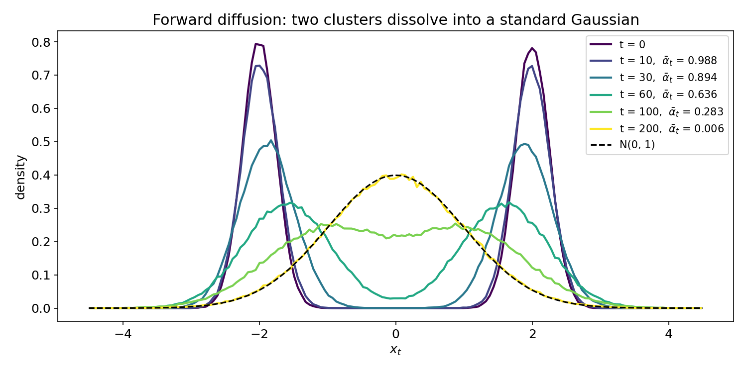
This is the theory half of a denoising diffusion model (DDPM), in one dimension so that every formula fits on a line. A data value x0 is corrupted step by step: at step t it is shrunk by αt and fresh Gaussian noise of variance 1−αt is added. You must show that after t steps xt is still a simple Gaussian around a shrunk x0, find what it converges to, compute the Kullback-Leibler divergence between two Gaussians, derive the exact "reverse" distribution of xt−1 given xt and x0, and finally show that the training objective collapses to a weighted squared error between the true noise and the noise predicted by a network. A last conceptual part asks how such a network should be told which time step it is working on.
How you are scored
50 points over 9 parts (5 or 10 points each), graded on complete derivations in a notebook. There is no dataset. We derived every formula by hand and then checked each one numerically in solution.py (Monte Carlo for the forward process, numerical integration for the KL, brute-force Bayes on a grid for the posterior, random tests for the final identities): all agree to 4 to 6 decimals.
part
result
3.1.1
A2=α1α2, B2=1−α1α2
3.1.2
xt∣x0∼N(αˉtx0,1−αˉt)
3.1.3
μt∣0→0, σt∣02→1 (when αˉt→0)
3.2.1
lnσqσp+2σp2σq2+(μq−μp)2−21
3.2.3
β~t=αt(1−αˉt)(αt−αˉt)(1−αt), μ~t below
3.2.4
μ~t=αt1(xt−1−αˉt1−αtϵˉt)
3.2.5
DKL=2(αt−αˉt)1−αt(ϵˉt−ϵθ(xt,t))2
The key idea
Everything rests on one fact: a linear combination of independent Gaussians is Gaussian, with means and variances that add. If ϵ,ϵ′ are independent N(0,1), then
aϵ+bϵ′∼N(0,a2+b2),soaϵ+bϵ′=a2+b2ϵˉ with ϵˉ∼N(0,1).
That turns t noisy steps into a single jump from x0 to xt (so training can sample any t directly), makes every distribution in the model Gaussian (so the KL is a closed formula), and lets the reverse mean be rewritten in terms of the noise (so the network only has to guess "which noise was added"). The schedule is designed so that each step preserves variance: Var[xt]=αtVar[xt−1]+(1−αt) equals 1 whenever Var[xt−1]=1.
Part 3.1: the forward process
3.1.1 Two steps
Write the two steps and substitute the first into the second:
using αtαˉt−1=αˉt. ϵˉt−1 depends only on ϵ1,…,ϵt−1, so it is independent of ϵt; the noise is Gaussian with variance αt−αtαˉt−1+1−αt=1−αˉt. This proves the claim with
At=αˉt,Bt=1−αˉt,xt∣x0∼N(αˉtx0,1−αˉt).
Monte Carlo check (400 000 chains, x0=1.7, linear schedule): at t=50 the empirical mean and variance are 1.4538 and 0.2690 against 1.4534 and 0.2691 predicted.
3.1.3 The limit
μt∣0=αˉtx0 and σt∣02=1−αˉt, so everything depends on limαˉt. The sequence αˉt is positive and decreasing (each factor is in (0,1)), so it converges. For any practical schedule, where the αt stay below some αmax<1, we have αˉt≤αmaxt→0, hence
t→∞limμt∣0=0,t→∞limσt∣02=1:
the chain forgets x0 entirely and xt tends to N(0,1), whatever the data. That is what makes generation possible: we can start the reverse process from pure noise.
A rigorous footnote worth knowing: 0<αt<1 alone is not quite enough. Since lnαˉt=∑slnαs and lnαs≈−(1−αs), we get αˉt→0 exactly when ∑t(1−αt)=∞. With αt=1−1/(t+1)2 the noise is summable and αˉt→1/2: the limit is then N(x0/2,1/2) and the data is never fully erased.
Part 3.2: the training objective
3.2.1 KL divergence between two Gaussians
By definition DKL(q∥p)=Ex∼q[lnq(x)−lnp(x)]. With the Gaussian density,
Take the expectation under q: Eq[(x−μq)2]=σq2, and writing x−μp=(x−μq)+(μq−μp), the cross term has zero mean, so Eq[(x−μp)2]=σq2+(μq−μp)2. Therefore
Interpretation: the mean is a weighted average of "where we are" (xt, rescaled) and "where we came from" (x0), weighted by how much each one tells us; the variance is smaller than both 1−αt and 1−αˉt−1, because two sources of information are combined. Brute-force check: normalising the product of the two densities on a grid of 400 001 points (for t=30, xt=0.4, x0=−1.2) gives mean 0.294652 and variance 0.006911, exactly the formulas. (For t=1, β~1=0: given x0, x0 is known; the formulas are meant for t≥2.)
3.2.4 In terms of the noise
From 3.1.2, x0=αˉtxt−1−αˉtϵˉt. Substituting into μ~t, the αˉt cancels in the second term:
The xt coefficients add to 1−αˉt, which cancels the denominator, and 1−αˉt1−αˉt=1−αˉt1:
μ~t=αt1(xt−1−αˉt1−αtϵˉt).
To go one step back, remove a well-chosen fraction of the noise that was put in, then undo the shrinking by αt.
3.2.5 The simplified objective
The network sees only xt and t, not x0, so it cannot compute ϵˉt; it predicts it, and we use the same formula: μθ(xt,t)=αt1(xt−1−αˉt1−αtϵθ(xt,t)). With σt2=β~t, the log term and the 2σt2β~t−21 terms of 3.2.2 vanish, leaving
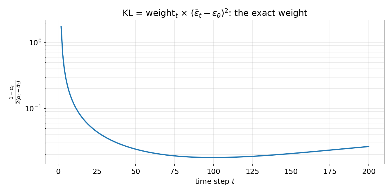
(Equivalently 2αt(1−αˉt−1)1−αt(ϵˉt−ϵθ)2.) Training a diffusion model is therefore regression on the noise: sample x0, t and ϵˉt, form xt=αˉtx0+1−αˉtϵˉt, and penalise the squared error of the network's guess. The weight in front depends only on t:
The exact KL puts most of the weight on the first few steps (fine details). Ho et al. found that simply dropping it, i.e. minimising E∥ϵˉt−ϵθ(xt,t)∥2 with t uniform, gives better samples: the "simple loss" every DDPM implementation uses.
Part 3.3: telling the network the time step
The same network must denoise slightly noisy inputs (small t) and almost pure noise (large t), so it needs t as an input. Since ϵθ must keep the shape (B,C,L0,…,LM−1), the standard design (as in DDPM's U-Net) is:
Represent t by a vector, not a raw integer. Use a sinusoidal embedding, as for positions in transformers: for a dimension d and frequencies ωk=10000−2k/d,
emb(t)=(sin(ω0t),cos(ω0t),…,sin(ωd/2−1t),cos(ωd/2−1t))∈Rd.
It is smooth in t, bounded, distinguishes all steps, and lets the network read both coarse and fine time differences. A learned lookup table nn.Embedding(T, d) also works when T is fixed. The embedding is then passed through a small MLP (for example Linear, SiLU, Linear) to get a learned time feature of shape (B,d′).
Inject it into every block, broadcast over space. In each residual block with C′ feature channels, a block-specific linear layer maps the time feature to (B,C′), which is reshaped to (B,C′,1,…,1) and added to the feature map (a per-channel bias that depends on t), or used as a per-channel scale and shift h↦(1+γ(t))h+β(t) (FiLM / adaptive normalisation). Broadcasting makes this work for any number M of spatial dimensions and keeps the output shape equal to the input shape.
Simpler alternatives, less effective: append t/T as an extra constant input channel (shape (B,1,L0,…)), or feed emb(t) as an extra token in a transformer backbone (as in DiT).
Injecting t at every block, rather than only at the input, matters because each layer's job (how much to smooth, how much detail to keep) depends on the noise level.