← Back to the problem

USA USAAIO 2026 · Correction by IOAI Training

Word Embedding Similarity and Low-Rank Approximation

This page gives the full approach. Read it once you have searched.

Metric
written + code answers (90 points)
Evaluated on
written answers
Our score
all 15 parts answered and verified
Expected level
bright -> lights check and correct proofs

Expected level reached

We solved the problem ourselves: downloaded the data, ran the experiments and measured the score below. The statement and data belong to their organisers.

The problem in brief

You take a short English text (three paragraphs about a seaside town), split it into lowercase tokens, and look up each distinct token in the pretrained GloVe embeddings, where every word is a vector of 100 numbers. After normalising the vectors you build the matrix SS of all pairwise cosine similarities, use it to find each word's closest neighbour, and then study SS with linear algebra: is it invertible, how does its eigen-decomposition relate to the SVD of the embedding matrix, what is its Frobenius norm, and how well can it be approximated with far fewer numbers. Fifteen short parts mix explanation, NumPy one-liners and proofs, with strict rules (no loops, no @, no np.linalg except for the SVD).

How you are scored

90 points over 15 parts (5 or 10 each). Code parts are checked by running them; "reasoning required" parts need a proof. Here is a summary of our answers, all checked by solution.py:

partanswer
5.1225 occurrences, then 158 distinct tokens
5.5simij∈[−1,1]\text{sim}_{ij} \in [-1, 1]
5.6S=WW⊤S = WW^\top
5.8all diagonal entries equal 1 (up to float32 rounding, within 4×10−74\times10^{-7})
5.9sim_dict["bright"] == "lights" reproduced
5.10not invertible: rank⁡S≤100<N=158\operatorname{rank} S \le 100 < N = 158
5.12Q=UQ = U, λ=(σ12,…,σ1002,0,…,0)\lambda = (\sigma_1^2, \dots, \sigma_{100}^2, 0, \dots, 0)
5.13∥S∥F=∑iσi4≈60.80\lVert S\rVert_F = \sqrt{\sum_i \sigma_i^4} \approx 60.80
5.14Wr=UrΣrW_r = U_r\Sigma_r, Sr=WrWr⊤S_r = W_rW_r^\top, error ∑i>rσi4/∑iσi4\sum_{i>r}\sigma_i^4 / \sum_i \sigma_i^4

First look at the data

The text has 225 tokens, all of which happen to be in GloVe's 400 000-word vocabulary, and 158 distinct ones. It was clearly written with groups of near-synonyms (walk, stroll, wander; happy, cheerful, pleased; tired, weary), so nearest neighbours should be meaningful. One surprise appears as soon as SS is drawn: 98 % of the off-diagonal similarities are positive (mean 0.34, minimum only −0.20-0.20, for "conversation" and "seabirds"). GloVe vectors are not spread evenly around the origin; they share a common direction. This will explain why the low-rank approximation works so well.
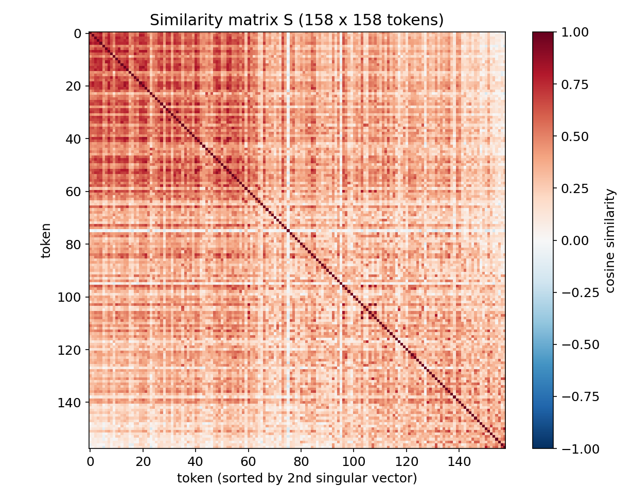
Heat map of the 158 by 158 similarity matrix. The diagonal is dark red (similarity 1); almost every other entry is pale to medium red, i.e. positive; there is hardly any blue.

Question by question

5.1 and 5.2: the two lengths and set

The first print(len(tokens)) counts every occurrence of every token that GloVe knows (225, repeated words such as "the" or "and" counted each time). tokens = list(set(tokens)) then builds a set, which keeps one copy of each distinct token, and converts it back to a list: 158 tokens. That is the answer to 5.2 too, with one caveat worth stating: a set has no order, so the order of the resulting list is arbitrary (it can change between Python runs). Our script sorts the list afterwards so that row nn of every matrix always refers to the same word.

5.3 and 5.4: the matrices

vectors_arr = np.array(vectors)                                        # (N, 100)
W = vectors_arr / np.sqrt((vectors_arr ** 2).sum(axis=1, keepdims=True))

keepdims=True makes the norms a column of shape (N,1)(N, 1), so broadcasting divides each row by its own norm.

5.5: the range

simij=v^(i)⊤v^(j)\text{sim}_{ij} = \hat v^{(i)\top}\hat v^{(j)} is the cosine of the angle between two unit vectors. By Cauchy-Schwarz, ∣v^(i)⊤v^(j)∣≤∥v^(i)∥ ∥v^(j)∥=1\lvert \hat v^{(i)\top}\hat v^{(j)}\rvert \le \lVert\hat v^{(i)}\rVert\,\lVert\hat v^{(j)}\rVert = 1, so simij∈[−1,1]\text{sim}_{ij} \in [-1, 1]: 1 for the same direction, −1-1 for opposite directions, 0 for orthogonal ones.

5.6 and 5.7: SS from WW

Entry (i,j)(i, j) of WW⊤WW^\top is row ii of WW dotted with row jj of WW, which is exactly simij\text{sim}_{ij}. So S=WW⊤S = WW^\top. Without @:

S = np.einsum("ik,jk->ij", W, W)        # or: S = np.dot(W, W.T)

5.8: the diagonal

print(np.diag(S)) shows values all equal to 1 (in float32 they range from 0.9999996 to 1.0000002). Interpretation: simii=∥v^(i)∥2=1\text{sim}_{ii} = \lVert\hat v^{(i)}\rVert^2 = 1, every word is perfectly similar to itself. This is a sanity check on the normalisation, and also a warning for the next part: the most similar token to any word is always itself.

5.9: nearest neighbours

So we mask the diagonal before taking the row-wise maximum:

S_off = S.copy()
np.fill_diagonal(S_off, -np.inf)
sim_dict = dict(zip(tokens, [tokens[j] for j in S_off.argmax(axis=1)]))

We get "bright": "lights" as the statement promises, and the neighbours are convincingly semantic: happy →\to pleased (0.74), walk →\to stroll, tired →\to weary, talked →\to spoke, night →\to evening (0.84), bread →\to baked, boats →\to fishermen. Note the last two: embeddings capture words that occur in the same contexts, not only synonyms.

5.10: is SS invertible?

No. S=WW⊤S = WW^\top with W∈RN×100W \in \mathbb{R}^{N \times 100}. Every column of SS is WW times a vector, so it lies in the column space of WW, which has dimension at most 100. Hence

rank⁡S≤rank⁡W≤100<158=N.\operatorname{rank} S \le \operatorname{rank} W \le 100 < 158 = N .

An N×NN \times N matrix of rank less than NN is singular. Concretely, there is a nonzero z∈RNz \in \mathbb{R}^N with W⊤z=0W^\top z = 0 (the 100×N100 \times N system W⊤z=0W^\top z = 0 has more unknowns than equations), and then Sz=W(W⊤z)=0Sz = W(W^\top z) = 0. In general: a Gram matrix of NN vectors in Rd\mathbb{R}^d can be invertible only if N≤dN \le d.

5.11 and 5.12: SVD of WW and spectral decomposition of SS

U, sigma, Vt = np.linalg.svd(W, full_matrices=True)    # U: N x N, sigma sorted decreasing
V = Vt.T

Substituting W=UΣV⊤W = U\Sigma V^\top:

S=WW⊤=UΣV⊤VΣ⊤U⊤=U (ΣΣ⊤) U⊤,S = WW^\top = U\Sigma V^\top V \Sigma^\top U^\top = U\,(\Sigma\Sigma^\top)\,U^\top ,

since V⊤V=IV^\top V = I. UU is orthonormal and ΣΣ⊤\Sigma\Sigma^\top is an N×NN\times N diagonal matrix with entries σ12≥⋯≥σ1002\sigma_1^2 \ge \dots \ge \sigma_{100}^2 followed by N−100=58N - 100 = 58 zeros. This is a spectral decomposition, already sorted in decreasing order:

Q = U
lam = np.concatenate([sigma ** 2, np.zeros(N - len(sigma))])

full_matrices=True matters: with the economy SVD, UU would be only N×100N \times 100 and not a square orthonormal QQ. (The 58 zero eigenvalues are another proof of 5.10.)

5.13: the Frobenius norm

The Frobenius norm satisfies ∥M∥F2=tr⁡(M⊤M)\lVert M\rVert_F^2 = \operatorname{tr}(M^\top M), and it is unchanged by orthonormal factors. Using 5.12 and the cyclic property of the trace:

∥S∥F2=tr⁡(S⊤S)=tr⁡(QΛQ⊤QΛQ⊤)=tr⁡(QΛ2Q⊤)=tr⁡(Λ2Q⊤Q)=∑iλi2=∑i=1100σi4.\lVert S\rVert_F^2 = \operatorname{tr}(S^\top S) = \operatorname{tr}(Q\Lambda Q^\top Q\Lambda Q^\top) = \operatorname{tr}(Q\Lambda^2 Q^\top) = \operatorname{tr}(\Lambda^2 Q^\top Q) = \sum_i \lambda_i^2 = \sum_{i=1}^{100}\sigma_i^4 .

So ∥S∥F=∑iσi4\lVert S\rVert_F = \sqrt{\sum_i \sigma_i^4}. Numerically both sides give 60.8046. A bonus identity: tr⁡S=∑iσi2=N\operatorname{tr} S = \sum_i \sigma_i^2 = N, because the diagonal of SS is all ones; indeed ∑iσi2=158.000\sum_i\sigma_i^2 = 158.000.

5.14: the best approximation with rNrN numbers

Keep the rr largest singular directions:

Wr=UrΣr∈RN×r(first r columns of U, scaled by σ1,…,σr),Sr=WrWr⊤=∑i=1rσi2 uiui⊤.W_r = U_r\Sigma_r \in \mathbb{R}^{N\times r} \quad(\text{first } r \text{ columns of } U, \text{ scaled by } \sigma_1,\dots,\sigma_r), \qquad S_r = W_rW_r^\top = \sum_{i=1}^{r}\sigma_i^2\, u_iu_i^\top .

By the same trace argument, S−Sr=∑i>rσi2uiui⊤S - S_r = \sum_{i>r}\sigma_i^2 u_iu_i^\top and

∥S−Sr∥F2∥S∥F2=∑i>rσi4∑iσi4.\frac{\lVert S - S_r\rVert_F^2}{\lVert S\rVert_F^2} = \frac{\sum_{i>r}\sigma_i^4}{\sum_{i}\sigma_i^4} .

Why this is the minimum: any Sr=WrWr⊤S_r = W_rW_r^\top has rank at most rr, and by the Eckart-Young theorem the closest rank-rr matrix to SS in Frobenius norm is obtained by keeping its rr largest eigen-components, which is exactly our SrS_r. Note that WrW_r is not "the first rr coordinates of the embeddings": that naive choice (renormalised) gives a relative error of 7.3 at r=1r = 1 and still 0.32 at r=50r = 50, against 0.088 and 0.0006 for the SVD.

5.15: the plot
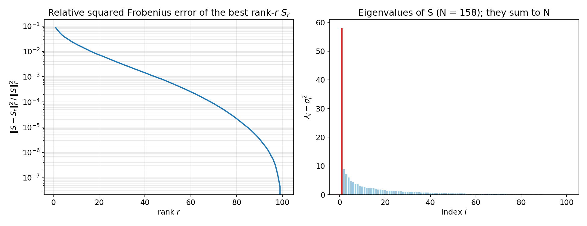
Left: the relative squared Frobenius error of the best rank-r approximation against r on a log scale, starting at 0.088 for r = 1 and falling steadily to essentially 0 at r = 100. Right: the 100 eigenvalues of S; the first is about 58, far above the second (about 8.9), and the rest decay slowly.

The key idea

A similarity matrix is a Gram matrix, so everything about it is governed by the SVD of the data matrix. S=WW⊤S = WW^\top immediately gives its rank (at most 100, hence singular), its eigenvectors (the left singular vectors of WW), its eigenvalues (σi2\sigma_i^2), its norm (∑σi4\sqrt{\sum\sigma_i^4}) and its best compressions (truncate the SVD).

The plot also tells a story about GloVe. A single rank-one term already captures 91 % of ∥S∥F2\lVert S\rVert_F^2. That first direction is almost exactly the average word vector (cosine 0.997 between the top right-singular vector and the mean of the rows of WW): all words share a common component, which is why nearly all similarities are positive. This "anisotropy" is common in embeddings, and subtracting the mean vector before computing similarities is a standard fix when one wants the remaining, more semantic directions to dominate. Because the error is measured with fourth powers of σi\sigma_i, this one dominant eigenvalue weighs enormously; reaching 1 % error needs r=17r = 17 and 5 % needs r=4r = 4.

The full solution

solution.py follows the starter code (only its imports), sorts the token list for reproducibility, and checks every claim with an assertion: S∈[−1,1]S\in[-1,1], QΛQ⊤=SQ\Lambda Q^\top = S and Q⊤Q=IQ^\top Q = I, the Frobenius identity, and the error formula of 5.14 against direct computation of ∥S−Sr∥F2\lVert S - S_r\rVert_F^2 for several rr. The plotting part of 5.15 is:

err = [(sigma[r:] ** 4).sum() / (sigma ** 4).sum() for r in range(1, 101)]
plt.plot(range(1, 101), err); plt.xlabel("r"); plt.ylabel("relative squared Frobenius error")

Results

checkvalue
tokens / distinct tokens225 / 158
diagonal of SS (float32)1 within 4×10−74\times10^{-7}
sim_dict["bright"]"lights"
rank⁡W\operatorname{rank} W100, so SS (158×158158\times158) is singular
∥S∥F\lVert S\rVert_F vs ∑σi4\sqrt{\sum\sigma_i^4}60.8046 vs 60.8046
relative error, best rank 1 / 5 / 10 / 20 / 500.088 / 0.037 / 0.019 / 0.0073 / 0.0006
same with naive "first rr coordinates"7.29 / 1.86 / 0.99 / 0.61 / 0.32
smallest rr for error ≤\le 5 % / 1 %4 / 17

What to remember

  • Cosine similarity of normalised rows is one matrix product: S=WW⊤S = WW^\top; mask the diagonal before searching for nearest neighbours.
  • A Gram matrix of NN vectors in Rd\mathbb{R}^d has rank at most dd, so it is singular whenever N>dN > d.
  • The SVD of WW hands you the eigen-decomposition of WW⊤WW^\top: same left vectors, squared singular values (and use full_matrices=True if you need a square QQ).
  • Frobenius norms and low-rank errors are sums over singular values, and truncating the SVD is optimal (Eckart-Young); cutting coordinates is not.
  • Look at the spectrum: one huge eigenvalue means a shared component (here, the mean word vector), which inflates all similarities.
Full code (solution.py)
"""USAAIO 2026 Round 1, Problem 5: word-embedding similarity, SVD and low rank.

Uses only the starter imports (gensim, requests, numpy, matplotlib), as the
problem requires; np.linalg is used only where the statement allows it (5.11).
Run:  python solution.py      (downloads GloVe-100, 128 MB, via gensim)
"""
import gensim.downloader as api
from gensim.utils import simple_preprocess
import requests
import numpy as np
import matplotlib
matplotlib.use("Agg")
import matplotlib.pyplot as plt

glove = api.load("glove-wiki-gigaword-100")
url = ("https://huggingface.co/datasets/usaaio-official/"
       "2026_USAAIO_Round1_public/raw/main/2026_USAAIO_Round1_NLP.txt")
text = requests.get(url).text

tokens = simple_preprocess(text)
print("all tokens:", len(tokens))
tokens = [token for token in tokens if token in glove]
print(len(tokens))                    # 5.1: occurrences (with repetitions)
tokens = list(set(tokens))
print(len(tokens))                    # 5.1: distinct tokens
tokens = sorted(tokens)               # (our addition) fixed order => reproducible
vectors = [glove[word] for word in tokens]

# 5.3  stack the N vectors as rows
vectors_arr = np.array(vectors, dtype=np.float64)        # (N, 100)
N, D = vectors_arr.shape

# 5.4  normalise each row (no np.linalg, no loop)
W = vectors_arr / np.sqrt((vectors_arr ** 2).sum(axis=1, keepdims=True))

# 5.6 / 5.7  S = W W^T   (one line, no @, no np.linalg, no loop)
S = np.einsum("ik,jk->ij", W, W)
assert S.min() >= -1 - 1e-12 and S.max() <= 1 + 1e-12   # 5.5: range [-1, 1]

# 5.8  diagonal
print("diagonal: min %.15f max %.15f" % (np.diag(S).min(), np.diag(S).max()))

# 5.9  nearest other token for every token
S_off = S.copy()
np.fill_diagonal(S_off, -np.inf)                          # exclude the token itself
best = S_off.argmax(axis=1)
sim_dict = dict(zip(tokens, [tokens[j] for j in best]))
print('sim_dict["bright"] =', sim_dict["bright"])
for w in ["happy", "walk", "sea", "tired", "bread", "night", "talked", "boats"]:
    print(f"  {w:>8s} -> {sim_dict[w]}   ({S_off[tokens.index(w)].max():.3f})")

# 5.10  rank(S) = rank(W) <= 100 < N  => S singular
print("N =", N, " rank(W) =", np.linalg.matrix_rank(W))

# 5.11  SVD of W
U, sigma, Vt = np.linalg.svd(W, full_matrices=True)       # U: (N,N), Vt: (100,100)
V = Vt.T
Sig = np.zeros((N, D)); np.fill_diagonal(Sig, sigma)
assert np.allclose(U.dot(Sig).dot(Vt), W)

# 5.12  spectral decomposition of S from the SVD
Q = U
lam = np.concatenate([sigma ** 2, np.zeros(N - D)]) if N > D else sigma ** 2
assert np.allclose(Q.dot(np.diag(lam)).dot(Q.T), S)
assert np.allclose(Q.T.dot(Q), np.eye(N))

# 5.13  Frobenius norm
fro = np.sqrt((S ** 2).sum())
print("||S||_F = %.6f, sqrt(sum sigma^4) = %.6f, trace check sum sigma^2 = %.6f (= N)"
      % (fro, np.sqrt((sigma ** 4).sum()), (sigma ** 2).sum()))
assert np.isclose(fro, np.sqrt((sigma ** 4).sum()))

# 5.14 / 5.15  best rank-r approximation: W_r = U_r Sigma_r, S_r = W_r W_r^T
rs = np.arange(1, D + 1)
err_formula = np.array([(sigma[r:] ** 4).sum() / (sigma ** 4).sum() for r in rs])
for r in [1, 2, 5, 10, 20, 50]:                           # direct check
    Wr = U[:, :r] * sigma[:r]
    Sr = Wr.dot(Wr.T)
    direct = ((S - Sr) ** 2).sum() / (S ** 2).sum()
    assert np.isclose(direct, err_formula[r - 1])
    # a naive alternative: keep the first r embedding coordinates, renormalise
    Wn = W[:, :r] / np.sqrt((W[:, :r] ** 2).sum(1, keepdims=True))
    naive = ((S - Wn.dot(Wn.T)) ** 2).sum() / (S ** 2).sum()
    print(f"r={r:3d}  optimal {err_formula[r-1]:.4f}   first-r-coords {naive:.4f}")
for t in [0.5, 0.2, 0.1, 0.05, 0.01]:
    print(f"smallest r with error <= {t}: {rs[err_formula <= t][0]}")

plt.rcParams.update({"font.size": 12})
fig, axes = plt.subplots(1, 2, figsize=(13, 5))
ax = axes[0]
ax.plot(rs, err_formula, color="#1f77b4", lw=2)
ax.set_xlabel("rank $r$")
ax.set_ylabel(r"$\|S - S_r\|_F^2 \,/\, \|S\|_F^2$")
ax.set_title("Relative squared Frobenius error of the best rank-$r$ $S_r$")
ax.set_yscale("log"); ax.grid(alpha=0.3, which="both")
ax = axes[1]
ax.bar(np.arange(1, D + 1), sigma ** 2, color="#9ecae1")
ax.bar([1], sigma[:1] ** 2, color="#d62728")
ax.set_xlabel("index $i$"); ax.set_ylabel(r"$\lambda_i = \sigma_i^2$")
ax.set_title(f"Eigenvalues of S (N = {N}); they sum to N")
fig.tight_layout()
fig.savefig("figures/low_rank_error.png", dpi=150)

# heat map of S, tokens ordered by the leading non-trivial singular vector
order = np.argsort(U[:, 1])
fig, ax = plt.subplots(figsize=(8.2, 6.5))
im = ax.imshow(S[np.ix_(order, order)], cmap="RdBu_r", vmin=-1, vmax=1)
fig.colorbar(im, ax=ax, fraction=0.046, label="cosine similarity")
ax.set_title(f"Similarity matrix S ({N} x {N} tokens)")
ax.set_xlabel("token (sorted by 2nd singular vector)"); ax.set_ylabel("token")
fig.tight_layout()
fig.savefig("figures/similarity_matrix.png", dpi=150)