Derivative of tanh and a Vectorised MSE Gradient

The problem in brief

Two small tasks that sit at the heart of training neural networks. First, differentiate the hyperbolic tangent $\tanh x = \frac{e^x - e^{-x}}{e^x + e^{-x}}$, with reasoning. Second, write a NumPy function that returns the gradient of the mean squared error of a linear model,

$$L(\theta) = \frac{1}{N}\sum_{n=0}^{N-1}\big(y[n] - \theta^\top X[n]\big)^2,$$

with respect to $\theta$, for X of shape $(N,d)$, y of shape $(N,)$ and theta of shape $(d,)$. The coding rules are strict: no extra imports, no autograd, nothing from np.linalg, no @, no .T, and no loop. This is Problem 4 of the 2026 USA AI Olympiad Round 1.

How you are scored

5 points for the derivative (the reasoning is required), 15 points for the function, and 0 for the function if any rule is broken. No official solution is published with the problem PDF. We checked both answers numerically: the derivative against central finite differences on $[-4,4]$ (largest gap $3\times10^{-11}$), and the gradient against finite differences ($5\times10^{-11}$) and against the textbook matrix formula ($10^{-15}$).

Question by question

4.1 The derivative of tanh

Write $u = e^x - e^{-x}$ and $v = e^x + e^{-x}$. Differentiating swaps them: $u' = e^x + e^{-x} = v$ and $v' = e^x - e^{-x} = u$. By the quotient rule,

$$\frac{d}{dx}\tanh x = \frac{u'v - uv'}{v^2} = \frac{v^2 - u^2}{v^2} = 1 - \Big(\frac{u}{v}\Big)^2 = 1 - \tanh^2 x .$$

Since $v^2 - u^2 = (u+v)(v-u) = 2e^x \cdot 2e^{-x} = 4$, the same result can also be written as

$$\frac{d}{dx}\tanh x = \frac{4}{(e^x + e^{-x})^2} = \frac{1}{\cosh^2 x}.$$

Both forms are worth knowing. The first, $1 - \tanh^2 x$, is the one used in backpropagation: the forward pass has already computed $a = \tanh x$, so the backward pass gets the local gradient $1 - a^2$ for free, without any new exponential.

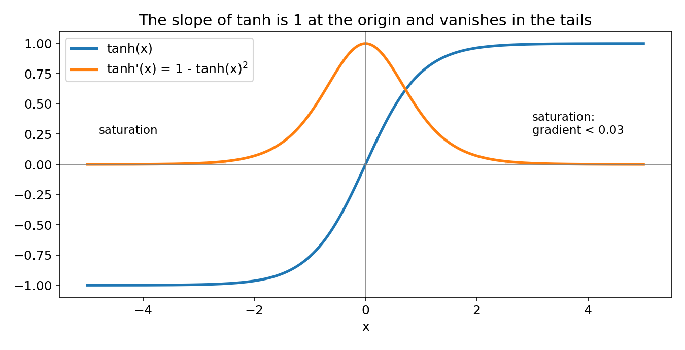
The picture explains why deep tanh networks were hard to train. The slope is at most 1 (at $x = 0$) and drops below 0.03 once $|x| > 2.5$. Backpropagation multiplies these factors layer after layer, so saturated units let almost no gradient through: the vanishing gradient problem that ReLU and careful initialisation later fixed.

4.2 The vectorised gradient

The maths. Let $r_n = y[n] - \theta^\top X[n]$ be the residual of sample $n$. By the chain rule, $\nabla_\theta\, r_n^2 = 2r_n\,\nabla_\theta r_n = -2 r_n X[n]$. Averaging over the samples,

$$\nabla_\theta L = -\frac{2}{N}\sum_{n=0}^{N-1} r_n\, X[n] .$$

In matrix form this is $-\frac{2}{N}X^\top(y - X\theta)$, but @ and .T are forbidden. That rule is the real exercise: we have to express both products with broadcasting and reductions.

• $X\theta$ is, for each row $n$, $\sum_j X[n,j]\,\theta[j]$. X * theta broadcasts theta (shape $(d,)$) over the $N$ rows, and np.sum(..., axis=1) sums each row. That gives the predictions, shape $(N,)$.
• $X^\top r$ is, for each column $j$, $\sum_n X[n,j]\, r_n$. residual[:, None] has shape $(N,1)$, so X * residual[:, None] scales row $n$ by $r_n$, and np.mean(..., axis=0) averages down the rows, which already contains the $1/N$.

import numpy as np

def my_fun_derivative(X, y, theta):
    residual = y - np.sum(X * theta, axis=1)              # (N,)
    return -2.0 * np.mean(X * residual[:, None], axis=0)  # (d,)

It uses no loop, no @, no .T and no np.linalg, and nothing is imported besides NumPy. The output has shape $(d,)$ as required. A one-line sanity check by hand: with $N = d = 1$, $X = 2$, $y = 3$, $\theta = 0.5$, the residual is $3 - 1 = 2$ and the gradient is $-2 \cdot 2 \cdot 2 = -8$, which the function returns.

Common pitfalls.

• Forgetting the factor 2, or the minus sign that comes from differentiating $y - \theta^\top X$ (the gradient then points uphill).
• Writing X * residual without [:, None]: shapes $(N,d)$ and $(N,)$ only broadcast if $d = N$, and then the result is silently wrong. Keep axes explicit.
• np.dot or np.matmul are not literally @, but they are matrix products and break the spirit of the rule; the broadcasting version is the safe answer.

What to remember

• $\tanh' = 1 - \tanh^2$: the derivative is written in terms of the function's own output, which is exactly what backpropagation needs.
• Saturating activations have tiny gradients in their tails: that is the root of vanishing gradients.
• The MSE gradient is "minus twice the average of residual times input": $-\frac{2}{N}X^\top(y - X\theta)$.
• Any matrix product can be rebuilt from broadcasting plus a sum over the shared axis. Thinking in terms of shapes, $(N,d) \times (d,) \to (N,)$, is the key skill.
• Always check a hand-derived gradient against finite differences.