IOAI Training: Learn AI by solving problems

The problem in brief

Problem 1 of the 2026 USA AI Olympiad Round 1 is a warm-up of five multiple-choice questions, each with one correct option out of five. They cover five ideas every ML practitioner must have at their fingertips: what "unsupervised" means, why the L1 penalty produces sparse models, how bias and variance move with model complexity, when the F1 score beats accuracy, and what UMAP preserves. Each is quick, but each distractor hides a classic misconception, so for every question we explain why the right answer is right and why the others are wrong. We also check the three quantitative claims with small experiments (solution.py).

How you are scored

10 points per part, 50 in total. Only the letter is graded. No official answer key was published with the problem PDF, so the answers below are our own derivations.

part	answer
1.1	C
1.2	B
1.3	D
1.4	D
1.5	B

Question by question

1.1 Which task is unsupervised? C

Supervised learning fits a map $x \mapsto y$ from examples whose target $y$ is given. Unsupervised learning only sees the inputs $x$ and must find structure in them by itself: clusters, low-dimensional directions, densities.

A (house prices from labelled prices) is supervised regression.
B (spam or not), D (malignant or benign) and E (labelled digit images) are supervised classification.
C groups customers "without predefined labels": that is clustering (k-means, for example), the textbook unsupervised task.

The trap is the word "grouping": classification also puts things into groups. What matters is whether the groups are given in advance.

1.2 L1 versus L2 at the same strength: B (L1 has fewer non-zero weights)

Both models minimise the squared error plus a penalty: $\lambda\sum_j |w_j|$ for A (Lasso), $\lambda\sum_j w_j^2$ for B (Ridge). Look at what each penalty does to a single weight near zero:

L2: the penalty's derivative, $2\lambda w_j$ , vanishes at 0. As a weight gets small, the push towards zero gets small too, so the weight shrinks but almost never lands exactly on 0.
L1: the penalty's slope is $\pm\lambda$ even arbitrarily close to 0. If the data's gradient on $w_j$ is smaller than $\lambda$ in absolute value, then $w_j = 0$ is optimal: the weight is clipped to exactly zero ("soft thresholding", $w = \operatorname{sign}(z)\max(|z|-\lambda, 0)$ in one dimension).

Geometrically, the L1 ball is a diamond whose corners lie on the axes, and the error's level sets usually first touch it at a corner, where some coordinates are 0. The L2 ball is round and has no corners.

So A typically has fewer non-zero weights. D is false (L1 does produce zeros). E is too pessimistic: it is not guaranteed for every dataset, but the question asks what is "most likely true".

Check. 50 features, 5 of them useful, 200 samples. With the penalty strengths we tried (0.05, 0.2, 0.5), Lasso keeps 15 non-zero weights at the weakest strength and exactly the 5 useful ones at the two stronger strengths, while Ridge keeps all 50 every time.

1.3 Bias and variance as complexity grows: D

For squared error, the expected test error at a point splits into

\mathbb{E}\big[(\hat f(x) - y)^2\big] = \underbrace{\big(\mathbb{E}[\hat f(x)] - f(x)\big)^2}_{\text{bias}^2} + \underbrace{\operatorname{Var}[\hat f(x)]}_{\text{variance}} + \sigma^2_{\text{noise}},

where the expectation is over the random training set. A more flexible model (a higher polynomial degree) can follow the true function more closely, so its average prediction is closer to the truth: bias falls. But it also follows the noise of the particular sample it was trained on, so its predictions change a lot from one training set to another: variance rises. That trade-off is why the test error is U-shaped. The other options contradict this: A and B move both terms together, C ignores the effect of complexity, and E has it backwards.

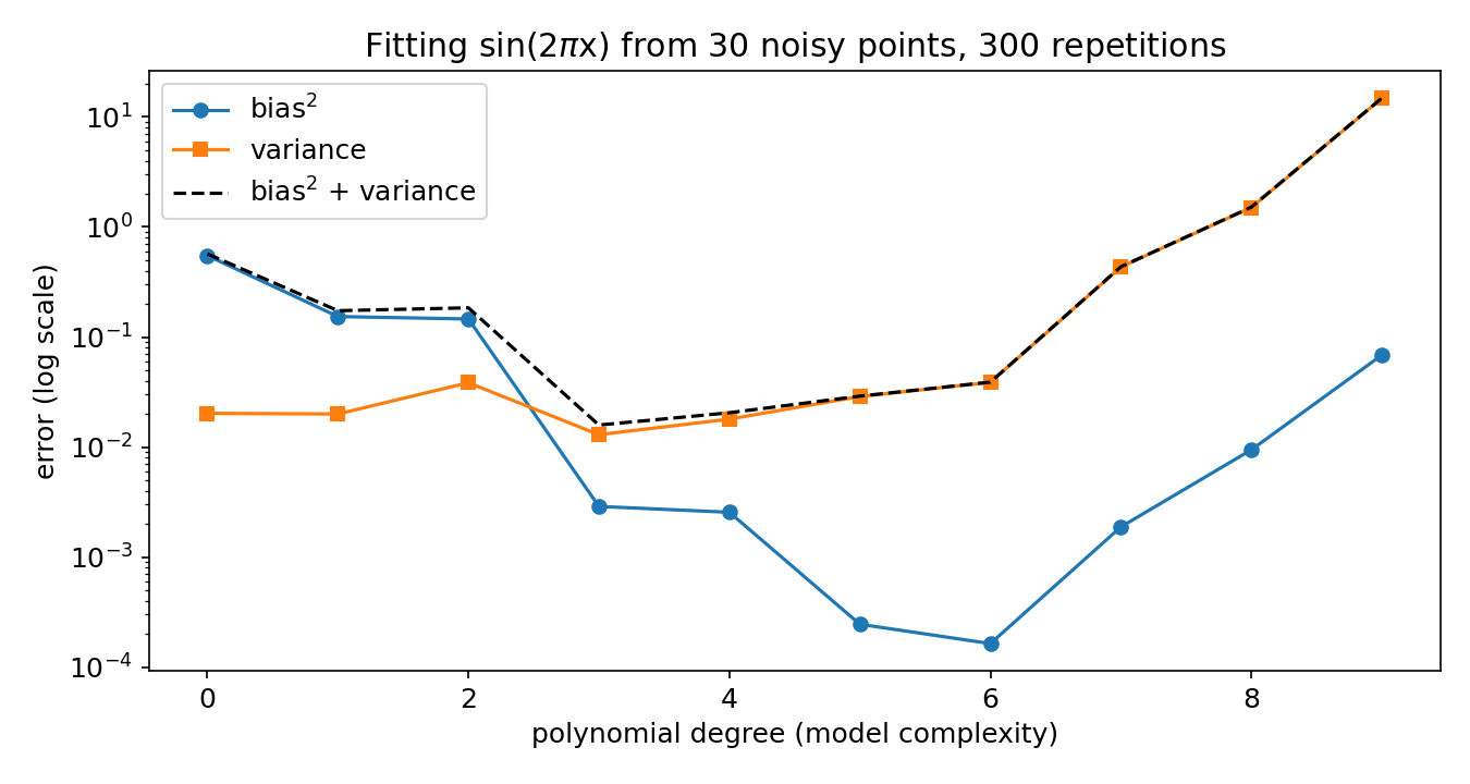
Bias squared and variance against polynomial degree

We fitted polynomials of degree 0 to 9 to 300 independent training sets of 30 noisy points of $\sin(2\pi x)$ . Bias² falls from 0.55 (a constant) to about 0.003 at degree 3 and stays tiny, while the variance grows from 0.02 to 0.43 at degree 7 and 14.8 at degree 9. The sum is smallest around degree 3 to 5.

1.4 When is F1 preferred to accuracy? D, on highly imbalanced data

With 1 % positives, a model that always answers "negative" is 99 % accurate and completely useless. F1 is the harmonic mean of precision and recall on the positive class:

F_1 = \frac{2PR}{P + R}, \qquad P = \frac{TP}{TP + FP}, \quad R = \frac{TP}{TP + FN}.

It ignores the (huge) number of true negatives, and it is 0 for the "always negative" model, which has $TP = 0$ . Our check, with 10 000 labels and about 1 % positives: accuracy 0.989, F1 0.000. Dataset size (A), linearity (C) and the number of features (E) have nothing to do with the choice, and on balanced classes (B) accuracy is perfectly informative.

1.5 What does UMAP do? B, it favours local neighbourhoods

UMAP (Uniform Manifold Approximation and Projection) builds a weighted $k$ -nearest-neighbour graph of the data, in which each point's distances are rescaled by the distance to its own nearest neighbours. It then looks for a low-dimensional layout whose own neighbour graph matches the first one, by minimising a fuzzy cross-entropy between the two graphs' edge weights. Because only neighbour relations enter the loss, local neighbourhoods are preserved well, while distances between far-apart clusters and cluster sizes carry little meaning.

A: no non-linear embedding into fewer dimensions can preserve all pairwise distances in general; UMAP does not even try.
C: UMAP is non-linear. That is its point, compared with PCA.
D: minimising reconstruction error is what PCA (and autoencoders) do; UMAP has no decoder.
E: nothing forces equal sizes. If anything, cluster areas in a UMAP plot should not be read as cluster sizes.

What to remember

Supervised means the targets are given; "grouping" without labels is clustering.
L1 has a constant slope at zero, so it sets weights exactly to zero; L2's slope vanishes there, so it only shrinks them.
More complexity means less bias and more variance; the sweet spot minimises their sum.
On imbalanced data, accuracy rewards the majority class; use F1, precision and recall, or PR-AUC.
UMAP and t-SNE plots show who is next to whom, not how far apart clusters are or how big they are.

"""USAAIO 2026 Round 1, Problem 1: small experiments that confirm each multiple-choice answer.

1.2  L1 (Lasso) vs L2 (Ridge) at the same strength: count exactly-zero weights.
1.3  Polynomial regression of growing degree: bias^2 and variance estimated over many datasets.
1.4  A 'always predict the majority class' model on imbalanced data: accuracy vs F1.
1.5  UMAP is not installed by default; we illustrate the local-vs-global point with t-SNE-free
     maths in the correction instead (no code needed).
Writes figures/bias_variance.png.
"""
import numpy as np, matplotlib
matplotlib.use('Agg'); import matplotlib.pyplot as plt
from sklearn.linear_model import Lasso, Ridge
from sklearn.metrics import accuracy_score, f1_score

rng = np.random.default_rng(0)

# ---- 1.2 sparsity: 50 features, only 5 matter
X = rng.normal(size=(200, 50)); w = np.zeros(50); w[:5] = [3, -2, 1.5, 1, -1]
y = X @ w + rng.normal(scale=0.5, size=200)
for lam in [0.05, 0.2, 0.5]:
    a = Lasso(alpha=lam).fit(X, y); b = Ridge(alpha=lam * 200).fit(X, y)   # same penalty scale
    print(f'1.2  lambda={lam}: non-zero weights  L1 = {np.sum(a.coef_ != 0):2d}   L2 = {np.sum(b.coef_ != 0):2d}')

# ---- 1.3 bias-variance for polynomial degree
f = lambda x: np.sin(2 * np.pi * x)
xs = np.linspace(0.05, 0.95, 200); degrees = range(0, 10); B2, V = [], []
for d in degrees:
    preds = []
    for _ in range(300):                                   # 300 independent training sets of 30 points
        x = rng.uniform(0, 1, 30); t = f(x) + rng.normal(scale=0.3, size=30)
        preds.append(np.polyval(np.polyfit(x, t, d), xs))
    P = np.array(preds)
    B2.append(np.mean((P.mean(0) - f(xs)) ** 2)); V.append(np.mean(P.var(0)))
    print(f'1.3  degree {d:2d}: bias^2 = {B2[-1]:.4f}  variance = {V[-1]:.4f}')
plt.rcParams.update({'font.size': 12})
fig, ax = plt.subplots(figsize=(9, 4.8))
ax.semilogy(list(degrees), B2, 'o-', label='bias$^2$')
ax.semilogy(list(degrees), V, 's-', label='variance')
ax.semilogy(list(degrees), np.array(B2) + np.array(V), 'k--', label='bias$^2$ + variance')
ax.set_xlabel('polynomial degree (model complexity)'); ax.set_ylabel('error (log scale)')
ax.set_title('Fitting sin(2$\\pi$x) from 30 noisy points, 300 repetitions'); ax.legend()
plt.tight_layout(); plt.savefig('figures/bias_variance.png', dpi=150, facecolor='white')

# ---- 1.4 accuracy vs F1 on imbalanced labels (1 % positives)
yt = (rng.random(10000) < 0.01).astype(int); yp = np.zeros_like(yt)
print(f'1.4  always-negative model: accuracy = {accuracy_score(yt, yp):.3f}, '
      f'F1 = {f1_score(yt, yp, zero_division=0):.3f}')

Machine Learning Concepts (Multiple Choice)