Matrix of a Linear Map and Rank-One Decomposition

The problem in brief

A linear map takes a vector $x = (x_0, x_1, x_2, x_3)$ of $\mathbb{R}^4$ to the vector $(x_2 - x_3,\ x_3,\ x_0 + 2x_1)$ of $\mathbb{R}^3$. First you must write down the $3 \times 4$ matrix $A$ of this map. Then you must express $A$ as a sum of $I$ outer products $u^{(i)} v^{(i)\top}$ (rank-one matrices), giving $I$ and every vector, with a justification. This is a short linear-algebra warm-up from Round 1 of the 2026 USA AI Olympiad, but the second part hides the idea behind PCA, SVD and low-rank compression of neural networks.

How you are scored

Each part is worth 5 points. Part 3.1 only needs the matrix. Part 3.2 needs $I$, the vectors and the reasoning. The decomposition is not unique, so a good answer gives one valid decomposition, checks it, and explains why its number of terms is the natural one.

Our answers (all verified in solution.py):

$$A = \begin{pmatrix} 0 & 0 & 1 & -1 \\ 0 & 0 & 0 & 1 \\ 1 & 2 & 0 & 0 \end{pmatrix}, \qquad I = 3 \ (\text{the rank of } A,\ \text{the smallest possible}).$$

Question by question

3.1 The matrix

The cleanest way to read a matrix off a linear map is: column $j$ of $A$ is the image of the $j$-th basis vector $e_j$, because $A e_j$ picks out column $j$. Plug in each basis vector:

input	$x_2 - x_3$	$x_3$	$x_0 + 2x_1$	column
$e_0 = (1,0,0,0)$	0	0	1	$(0,0,1)^\top$
$e_1 = (0,1,0,0)$	0	0	2	$(0,0,2)^\top$
$e_2 = (0,0,1,0)$	1	0	0	$(1,0,0)^\top$
$e_3 = (0,0,0,1)$	$-1$	1	0	$(-1,1,0)^\top$

Equivalently, row $i$ of $A$ lists the coefficients of the $i$-th output: the first output is $0x_0 + 0x_1 + 1x_2 - 1x_3$, and so on. Either way,

$$A = \begin{pmatrix} 0 & 0 & 1 & -1 \\ 0 & 0 & 0 & 1 \\ 1 & 2 & 0 & 0 \end{pmatrix}.$$

Quick check with $x = (1,1,1,1)$: $Ax = (0, 1, 3)$, and indeed $x_2 - x_3 = 0$, $x_3 = 1$, $x_0 + 2x_1 = 3$.

3.2 A sum of rank-one matrices

What an outer product is. For $u \in \mathbb{R}^3$ and $v \in \mathbb{R}^4$, the matrix $u v^\top$ has entries $(u v^\top)_{jk} = u_j v_k$: every row is a multiple of $v^\top$ and every column is a multiple of $u$. It has rank 1 (if $u, v \neq 0$). Acting on $x$ it gives $u\,(v^\top x)$: "measure $x$ along $v$, then output that amount in direction $u$".

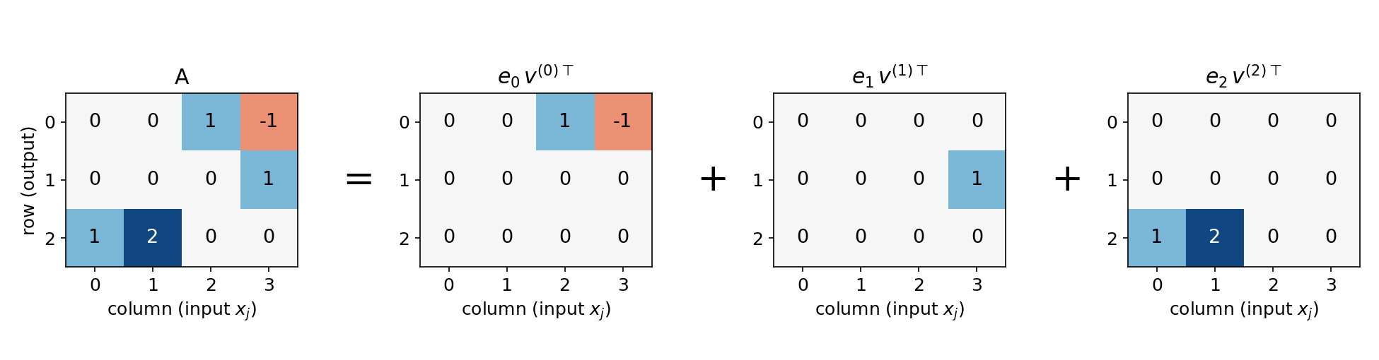
A decomposition with $I = 3$ terms (row form). Write $A$ as the sum of its rows placed in their own position. With $e_0, e_1, e_2$ the standard basis of $\mathbb{R}^3$,

$$A = \sum_{i=0}^{2} e_i\, (\text{row}_i A)^\top ,$$

that is,

$$u^{(0)} = \begin{pmatrix}1\\0\\0\end{pmatrix},\ v^{(0)} = \begin{pmatrix}0\\0\\1\\-1\end{pmatrix};\quad u^{(1)} = \begin{pmatrix}0\\1\\0\end{pmatrix},\ v^{(1)} = \begin{pmatrix}0\\0\\0\\1\end{pmatrix};\quad u^{(2)} = \begin{pmatrix}0\\0\\1\end{pmatrix},\ v^{(2)} = \begin{pmatrix}1\\2\\0\\0\end{pmatrix}.$$

Reading it as a map: term $i$ computes output number $i$ (namely $v^{(i)\top}x$) and writes it in slot $i$ (direction $e_i$). This is exactly how the map was defined.

Why no decomposition uses fewer than 3 terms. Every column of $\sum_{i<I} u^{(i)} v^{(i)\top}$ is a combination of $u^{(0)}, \dots, u^{(I-1)}$, so the column space has dimension at most $I$:

$$\operatorname{rank}\Big(\sum_{i=0}^{I-1} u^{(i)} v^{(i)\top}\Big) \le I .$$

Now $\operatorname{rank} A = 3$: columns 0, 2 and 3 are $(0,0,1)$, $(1,0,0)$ and $(-1,1,0)$, and

$$\det\begin{pmatrix} 0 & 1 & -1 \\ 0 & 0 & 1 \\ 1 & 0 & 0 \end{pmatrix} = 1 \neq 0,$$

so they are independent. Hence $I \ge 3$, and our decomposition is as short as possible. (Larger $I$ is always possible, for instance by splitting a term into two halves, which is why the natural answer is the minimal one.)

Other valid answers. Grouping by columns gives $A = \sum_j (\text{col}_j A)\, e_j^\top$ with 4 terms, but column 1 is twice column 0, so those two merge into $(0,0,1)^\top(1,2,0,0)$:

$$A = \begin{pmatrix}0\\0\\1\end{pmatrix}\!(1,2,0,0) + \begin{pmatrix}1\\0\\0\end{pmatrix}\!(0,0,1,0) + \begin{pmatrix}-1\\1\\0\end{pmatrix}\!(0,0,0,1).$$

The singular value decomposition gives a third, very special one, $A = \sum_i \sigma_i\, \tilde u^{(i)} \tilde v^{(i)\top}$ with orthonormal $\tilde u$'s and $\tilde v$'s. Here $AA^\top = \begin{pmatrix} 2 & -1 & 0\\ -1 & 1 & 0 \\ 0 & 0 & 5\end{pmatrix}$, whose eigenvalues are $5$ and $\frac{3 \pm \sqrt5}{2}$, so the singular values are $\sqrt5 \approx 2.236$, $\frac{1+\sqrt5}{2} \approx 1.618$ (the golden ratio) and $\frac{\sqrt5 - 1}{2} \approx 0.618$.

The key idea

A rank-one matrix $u v^\top$ is the simplest possible linear map: one input direction, one output direction. The rank of a matrix is the minimum number of such pieces needed to build it, and that is why the answer to "what is $I$?" is a theorem rather than a guess.

Among all decompositions, the SVD orders the pieces by importance (their $\sigma_i$). Keeping only the first $r$ terms gives the best possible rank-$r$ approximation (Eckart-Young theorem); the error left in Frobenius norm is $\sqrt{\sum_{i \ge r}\sigma_i^2}$. For our $A$, the best 2-term approximation still misses by $\sigma_2 \approx 0.618$, which confirms numerically that no two outer products reproduce $A$ exactly. This idea drives PCA, word-embedding compression, recommender systems and LoRA finetuning, where a weight update $\Delta W$ is forced to be a sum of a few outer products.

The full solution

solution.py builds $A$ by applying the map to $e_0, \dots, e_3$, checks $Ax = f(x)$ on 1000 random vectors, and verifies the three decompositions exactly:

A = np.column_stack([f(np.eye(4)[j]) for j in range(4)])     # column j = f(e_j)
U = [np.eye(3)[i] for i in range(3)]; V = [A[i] for i in range(3)]
assert np.array_equal(sum(np.outer(u, v) for u, v in zip(U, V)), A)
assert np.linalg.matrix_rank(A) == 3                           # so I = 3 is minimal

Results

check	outcome
$A$ from basis vectors, tested on 1000 random $x$	matches the map
row-form decomposition, $I = 3$	exact
column-form decomposition (columns 0 and 1 merged), $I = 3$	exact
SVD form, $\sigma = (\sqrt5,\ 1.618,\ 0.618)$	exact up to rounding
best possible 2-term approximation	error $0.618 > 0$, so $I = 2$ is impossible

What to remember

• Column $j$ of a matrix is the image of $e_j$. This turns "find the matrix of a linear map" into four substitutions.
• An outer product $u v^\top$ is a rank-one map: read along $v$, write along $u$. Any matrix is a sum of them (rows or columns give one immediately).
• The minimal number of rank-one terms equals the rank, because the rank of a sum of $I$ outer products is at most $I$.
• The SVD is the decomposition that sorts terms by importance, which is what makes truncation (PCA, low-rank compression, LoRA) optimal.