IOAI Training: Learn AI by solving problems

The problem in brief

You receive a table of 426 tumour biopsies, each described by 30 numeric measurements of the cell nuclei seen under a microscope (radius, texture, perimeter, area, smoothness and so on, each given as a mean, a standard error and a "worst" value). The label says whether the tumour is benign (1) or malignant (0). You must hand in a notebook that trains a classifier and exposes a function my_prediction(X_test) returning one label per row of a hidden test table. The twist is the rule: the only supervised model you may use is k-nearest neighbours. Everything else (preprocessing, feature engineering) is free, as long as it stays within scikit-learn, NumPy, pandas and matplotlib.

How you are scored

Predictions on the hidden test set are scored with the macro-averaged F1 score: compute the F1 score of each class, then average the two without weighting by class size,

F_1^{(c)} = \frac{2\,P_c R_c}{P_c + R_c}, \qquad \text{macro-}F_1 = \tfrac12\left(F_1^{(0)} + F_1^{(1)}\right),

where $P_c$ and $R_c$ are the precision and recall of class $c$ . Because the classes are unbalanced (268 benign, 158 malignant), macro-F1 punishes a model that neglects the smaller, malignant class much more than accuracy would. The grade also depends on the notebook running end to end and on the quality of the written reasoning. No threshold or reference score is published.

The hidden test labels are private, so every number below is measured on the training CSV only: 10 repetitions of stratified 5-fold cross-validation, plus one stratified 25 % hold-out. This data is a version of the well-known Wisconsin Diagnostic Breast Cancer set that ships with scikit-learn. Using that public copy to "check" test predictions would simply mean reading the answers, so we never touch it.

First look at the data

There are no missing values and no duplicates. The labels split 63 % / 37 %. The real surprise comes from the units. Perimeter should be roughly $2\pi \times$ radius, yet here the ratio $\text{perimeter} / (2\pi r)$ is about 1030 on every row: the three perimeter columns are stored about 1000 times too large. In the same way, the area columns are about 10 000 times too small ( $\text{area}/(\pi r^2) \approx 10^{-4}$ ). Whatever the reason (a deliberate trap or a unit mix-up), the result is that the features live on wildly different scales:

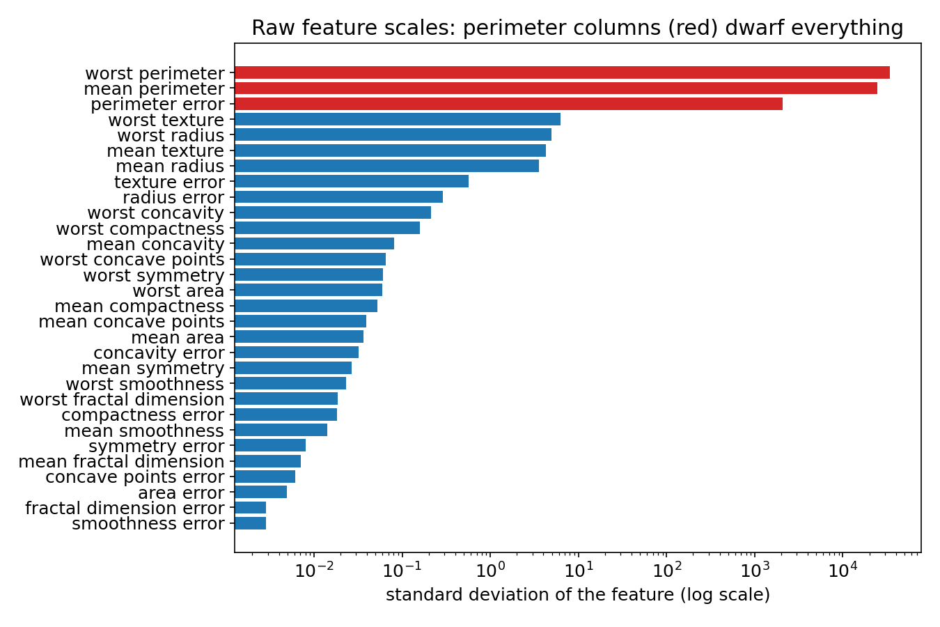
Standard deviation of each of the 30 raw features on a log scale. The three perimeter columns have standard deviations in the thousands or tens of thousands, the others range from 0.003 to about 6.

That matters enormously for k-NN, as we are about to see.

A first baseline

Out of the box, KNeighborsClassifier(k=5) on the raw columns gives a macro-F1 of 0.912 (10x5-fold CV). That is not bad, but it is misleading: the model is not really using 30 features. The Euclidean distance between two patients is

d(\mathbf{x}, \mathbf{x}') = \sqrt{\sum_{j=1}^{30} (x_j - x'_j)^2},

and a typical difference in "worst perimeter" is tens of thousands, against differences below 1 for most other features. The square root is almost exactly $\lvert x_{\text{worst perim}} - x'_{\text{worst perim}} \rvert$ plus a little of the other two perimeter columns: the "30-dimensional" model is in fact a 1-dimensional nearest neighbour on tumour size.

The key idea

k-NN has no weights to learn, so the distance itself is the model. In linear regression, a feature stored in the wrong unit gets its coefficient rescaled during training and nothing is lost. A neighbour classifier cannot do that: each feature counts in proportion to the square of its numeric range. Choosing how to scale the features is therefore choosing how much each feature counts.

The neutral choice is to standardise every column,

z_j = \frac{x_j - \mu_j}{\sigma_j},

with $\mu_j$ and $\sigma_j$ estimated on the training data only (inside the pipeline, so cross-validation folds never leak). Every feature then has variance 1 and contributes on the same footing. Two nice consequences:

The unit trap disappears completely. Multiplying a column by 1000 changes $\mu_j$ and $\sigma_j$ by the same factor, so $z_j$ does not move at all.
Texture, concavity and concave points, which carry information that size alone does not, finally get their say in the distance.

Once the scale is fixed, the remaining choice is $k$ . A small $k$ follows every noisy training point (high variance); a large $k$ averages over neighbours that are far away and may belong to the other class (high bias). Weighting votes by $1/d$ softens the dependence on $k$ .

Macro-F1 under 10x5-fold cross-validation as a function of k. The raw-feature curve stays near 0.90 to 0.91 for every k; the standardised curve rises to a peak of 0.963 at k = 7 and slowly decreases after.

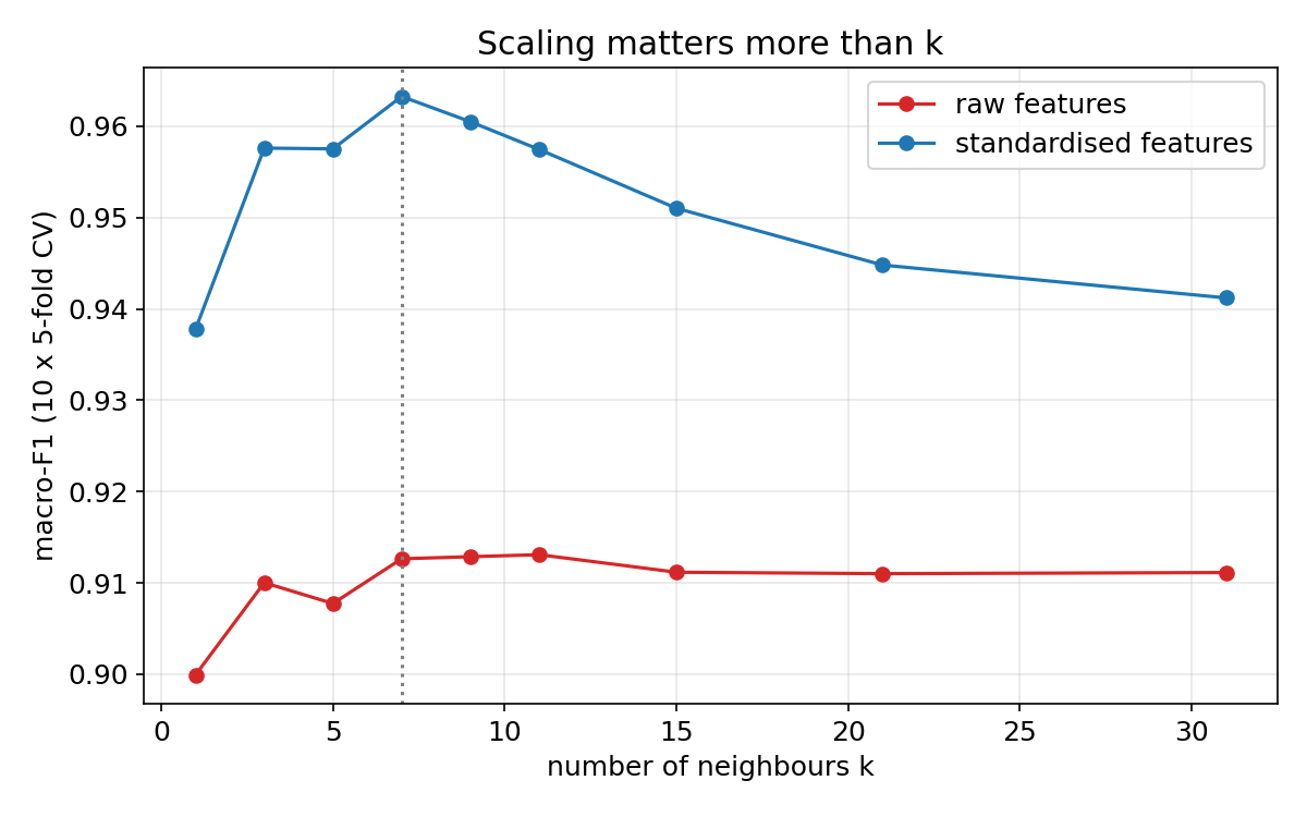
The picture says it all: no value of $k$ rescues the raw features, while any reasonable $k$ on standardised features beats them by about 5 points.

The full solution

Load the CSV, separate the 30 features from target.
Build make_pipeline(StandardScaler(), KNeighborsClassifier(n_neighbors=7, weights="distance")). Putting the scaler inside the pipeline guarantees that during cross-validation it is fitted on the training folds only.
Choose $k$ and the voting rule by repeated stratified CV (macro-F1), then confirm with a nested CV (grid search inside each outer fold) to measure the cost of tuning. The nested estimate (0.960) is close to the plain one (0.963), so the choice of $k = 7$ is not an overfitted lucky pick.
Refit on all 426 rows and define the inference function:

model = make_pipeline(StandardScaler(),
                      KNeighborsClassifier(n_neighbors=7, weights="distance")).fit(X, y)

def my_prediction(X_test):
    y_pred = model.predict(fix_units(X_test))
    return pd.Series(y_pred, index=X_test.index, name="target")

fix_units is a small defensive step: if the hidden test file happened to store perimeters in the usual unit (ratio to $2\pi r$ near 1 instead of 1000), it converts them to the training units before predicting. With standardisation fitted on training data, a test column in a different unit would otherwise be shifted by thousands of standard deviations. If the test file is in the same units as the training file, as is most likely, the function does nothing. Selecting the columns by name (X_test[COLS]) also protects against a reordered test table.

Results

approach	macro-F1 (10x5-fold CV)
raw features, k = 5	0.912
raw features, best k (11)	0.913
standardised, k = 1	0.938
standardised, k = 5	0.958
standardised, k = 7, distance weights (submitted)	0.963
standardised, k = 21	0.945
standardised + Manhattan distance, k = 9	0.957
log transform + standardise, k = 9	0.953
quantile transform to Gaussian, k = 15	0.959
standardise + PCA (5 components), k = 9	0.958
standardise + PCA (2 components), k = 9	0.925
standardise + 10 best features by ANOVA F, k = 9	0.932
standardise + forward feature selection (10 features), nested	0.955
standardise + NCA metric learning, k = 9	0.953
nested CV, grid over k, weights, p	0.960
submitted model on a 25 % stratified hold-out	0.970

The fold-to-fold standard deviation is about 0.02, so every standardised variant between 0.955 and 0.963 is statistically tied. The fancier ideas (feature selection, PCA, learned metrics) did not help: with only 426 rows, each extra choice adds variance, and the 30 standardised features are already informative and not very noisy. Throwing features away hurt the most, because many of them are correlated measurements of the same nuclei and averaging over them makes the distance more stable.

What to remember

For distance-based models (k-NN, k-means, SVM with RBF kernel), scaling is part of the model. A feature's influence grows with the square of its range; standardise unless you have a reason to weight features differently.
Always sanity-check units with domain relations (perimeter against radius, area against radius squared). A one-line ratio revealed that three columns were 1000 times too large.
Fit preprocessing inside the pipeline so cross-validation never sees statistics from the validation fold, and make the inference function robust to column order and unit surprises.
With small data, report a mean and a spread over repeated CV, and prefer the simplest model inside the noise band: differences of 0.005 in macro-F1 here are noise.
A public copy of a competition dataset is not a test set. Evaluate on your own held-out split; anything else is reading the answer key.

"""USAAIO 2026 Round 1, Problem 9: breast-cancer classification with k-NN.

Pipeline: StandardScaler -> KNeighborsClassifier(k=7, distance weights).
Evaluation: repeated stratified 5-fold CV on the public training CSV and one
stratified 25 % hold-out (the official test labels are private; we never use
any outside copy of the dataset as a test set).
Run:  python solution.py   (downloads the 100 KB training CSV)
"""
import warnings
import numpy as np
import pandas as pd
import matplotlib
matplotlib.use("Agg")
import matplotlib.pyplot as plt
from sklearn.neighbors import KNeighborsClassifier
from sklearn.pipeline import make_pipeline
from sklearn.preprocessing import StandardScaler
from sklearn.model_selection import (RepeatedStratifiedKFold, cross_val_score,
                                     train_test_split)
from sklearn.metrics import f1_score

warnings.filterwarnings("ignore")
URL = ("https://huggingface.co/datasets/usaaio-official/"
       "2026_USAAIO_Round1_public/raw/main/2026_USAAIO_Round1_breast_cancer_train.csv")

df = pd.read_csv(URL)
X = df.drop("target", axis=1)
y = df["target"]
print(X.shape, y.value_counts().to_dict())          # (426, 30) {1: 268, 0: 158}

# ------------------------------------------------------------------ 1. look
# The perimeter columns are stored about 1000x too big and the area columns
# about 10000x too small (perimeter / (2*pi*radius) ~ 1030 on every row).
ratio = X["mean perimeter"] / (2 * np.pi * X["mean radius"])
print("perimeter/(2 pi r):", ratio.median().round(1))
spread = X.std().sort_values(ascending=False)
print("largest std:", spread.head(4).round(1).to_dict())

# ---------------------------------------------- 2. compare models honestly
cv = RepeatedStratifiedKFold(n_splits=5, n_repeats=10, random_state=0)

def cv_f1(model):
    s = cross_val_score(model, X, y, cv=cv, scoring="f1_macro", n_jobs=4)
    return s.mean(), s.std()

ks = [1, 3, 5, 7, 9, 11, 15, 21, 31]
raw_curve, std_curve = [], []
for k in ks:
    raw_curve.append(cv_f1(KNeighborsClassifier(k, weights="distance"))[0])
    std_curve.append(cv_f1(make_pipeline(StandardScaler(),
                       KNeighborsClassifier(k, weights="distance")))[0])
    print(f"k={k:2d}  raw {raw_curve[-1]:.4f}   scaled {std_curve[-1]:.4f}")

# ------------------------------------------------------- 3. final pipeline
def make_model():
    return make_pipeline(StandardScaler(),
                         KNeighborsClassifier(n_neighbors=7, weights="distance"))

m, s = cv_f1(make_model())
print(f"final model, 10x5-fold CV macro-F1 = {m:.4f} +- {s:.4f}")

Xtr, Xho, ytr, yho = train_test_split(X, y, test_size=0.25, stratify=y,
                                      random_state=42)
ho = f1_score(yho, make_model().fit(Xtr, ytr).predict(Xho), average="macro")
print(f"final model, 25 % hold-out macro-F1 = {ho:.4f}")

model = make_model().fit(X, y)                      # refit on all 426 rows
COLS = list(X.columns)
TRAIN_RATIO = float(ratio.median())


def fix_units(Xt):
    """Defensive: bring test units in line with training units if the hidden
    test file was stored with the usual (uncorrupted) perimeter/area units."""
    Xt = Xt[COLS].astype(float).copy()
    r = (Xt["mean perimeter"] / (2 * np.pi * Xt["mean radius"])).median()
    if r < TRAIN_RATIO / 100:                        # perimeters look normal
        for c in COLS:
            if "perimeter" in c:
                Xt[c] *= 1000
            if "area" in c:
                Xt[c] /= 10000
    return Xt


def my_prediction(X_test):
    y_pred = model.predict(fix_units(X_test))
    return pd.Series(y_pred, index=X_test.index, name="target")


print(my_prediction(X.head(5)).tolist(), y.head(5).tolist())

# ---------------------------------------------------------------- figures
plt.rcParams.update({"font.size": 12})
fig, ax = plt.subplots(figsize=(9, 6))
top = X.std().sort_values()
colors = ["#d62728" if "perimeter" in c else "#1f77b4" for c in top.index]
ax.barh(top.index, top.values, color=colors)
ax.set_xscale("log")
ax.set_xlabel("standard deviation of the feature (log scale)")
ax.set_title("Raw feature scales: perimeter columns (red) dwarf everything")
fig.tight_layout()
fig.savefig("figures/feature_scales.png", dpi=150)

fig, ax = plt.subplots(figsize=(8, 5))
ax.plot(ks, raw_curve, "o-", label="raw features", color="#d62728")
ax.plot(ks, std_curve, "o-", label="standardised features", color="#1f77b4")
ax.axvline(7, ls=":", color="grey")
ax.set_xlabel("number of neighbours k")
ax.set_ylabel("macro-F1 (10 x 5-fold CV)")
ax.set_title("Scaling matters more than k")
ax.legend()
ax.grid(alpha=0.3)
fig.tight_layout()
fig.savefig("figures/f1_vs_k.png", dpi=150)

Breast Cancer Classification with k-NN