Slovakia OAI 2026 · Correction by IOAI Training

Recognising Grains (Dry Bean Varieties)

This page gives the full approach. Read it once you have searched.

Metric: macro F1
Evaluated on: held-out validation (official test labels are private)
Our score: 0.933 macro F1 (92.2 % accuracy)
Expected level: no score threshold: report graded by rubric

We solved the problem ourselves: downloaded the data, ran the experiments and measured the score below. The statement and data belong to their organisers.

The problem in brief

A camera photographs dry beans one by one, and image analysis turns each bean's silhouette into 16 numbers: its area, perimeter, the lengths of its long and short axes, and several shape ratios built from them. You get 13 611 beans from seven Turkish varieties (Barbunya, Bombay, Cali, Dermason, Horoz, Seker, Sira) and must predict the variety. The real twist is that the organisers want more than a good score: you have to build decision trees, compare them with tree ensembles, use PCA to look at the data, pull human-readable rules out of the tree, explain specific mistakes, and finally design a cheap sorting machine that measures only 3 to 5 quantities.

The data is the public UCI Dry Bean dataset. The organisers' online judge (which needs a login) holds a private train/test split scored with F1. We did not use it: we rebuilt the setup on the public data with a stratified 80/20 split (10 834 training beans, 2 709 held-out beans), made every modelling choice by cross-validation on the training part, and touched the held-out part only to report the final numbers. All scores below are on our own held-out split, not on the official test set, whose labels are private.

How you are scored

There are two layers. The written report is marked out of 100 points: 30 for correct data preparation and implementation, 20 for the decision-tree modelling, 15 for the comparison with ensembles, 15 for meaningful use of PCA, and 20 for interpretation and clarity. The judge's numerical score, and the metric the statement asks you to report, is the macro F1-score. For each class $c$ , with precision $P_c$ and recall $R_c$ :

F1_c = \frac{2\,P_c R_c}{P_c + R_c}, \qquad \text{macro-}F1 = \frac{1}{7}\sum_{c=1}^{7} F1_c .

Every variety counts equally, whatever its size. Bombay, the rarest class (3.8 % of beans), weighs as much as Dermason (26 %). A model that never predicts Bombay loses a full seventh of the score, even though its accuracy hardly moves. Keep that in mind: it explains one of the most surprising results below.

What to aim for. The organisers publish no threshold. The natural reference is the paper that introduced the dataset (Koklu and Ozkan, Computers and Electronics in Agriculture, 2020), which evaluates its models with 10-fold cross-validation. Rerunning that protocol ourselves, our SVM reaches 93.2 % accuracy and our gradient-boosted trees 93.0 %, which suggests the ceiling of this dataset sits around 93 % accuracy, or about 0.93 to 0.94 macro F1.

First look at the data

Cleaning. Nothing is missing. All values are physically plausible (no negative lengths, no aspect ratio below 1). There are, however, 68 exact duplicate rows, all of them Horoz. If you keep them, a bean and its copy can land on opposite sides of the split, and the model is then tested on a bean it has already seen. We drop them, which leaves 13 543 beans.

The 16 features are really about 6 measurements. Checking the formulas numerically (they agree to machine precision) shows that most features are just algebra on the area $A$ , perimeter $P$ , major axis $L$ and minor axis $l$ :

\text{roundness} = \frac{4\pi A}{P^2}, \quad \text{Compactness} = \frac{\sqrt{4A/\pi}}{L}, \quad \text{ShapeFactor1} = \frac{L}{A}, \quad \text{ShapeFactor3} = \text{Compactness}^2, \quad \text{ShapeFactor4} = \frac{A}{\pi L l / 4}.

One small surprise: ShapeFactor2 is $A/L^3$ , not the $l/A$ given in the original paper. Only ConvexArea and Extent bring in information from outside these four measurements. That redundancy shows up in the correlations: Area and ConvexArea correlate at 0.9999, Compactness and ShapeFactor3 at 0.999, and Perimeter and EquivDiameter at 0.991. A bean has two kinds of property, its size and its shape, and every feature is mostly one, the other, or a mix of both.

PCA. PCA is sensitive to units (Area is around $10^5$ , ShapeFactor2 around $10^{-3}$ ), so we standardise first, fitting the scaler on the training part only.

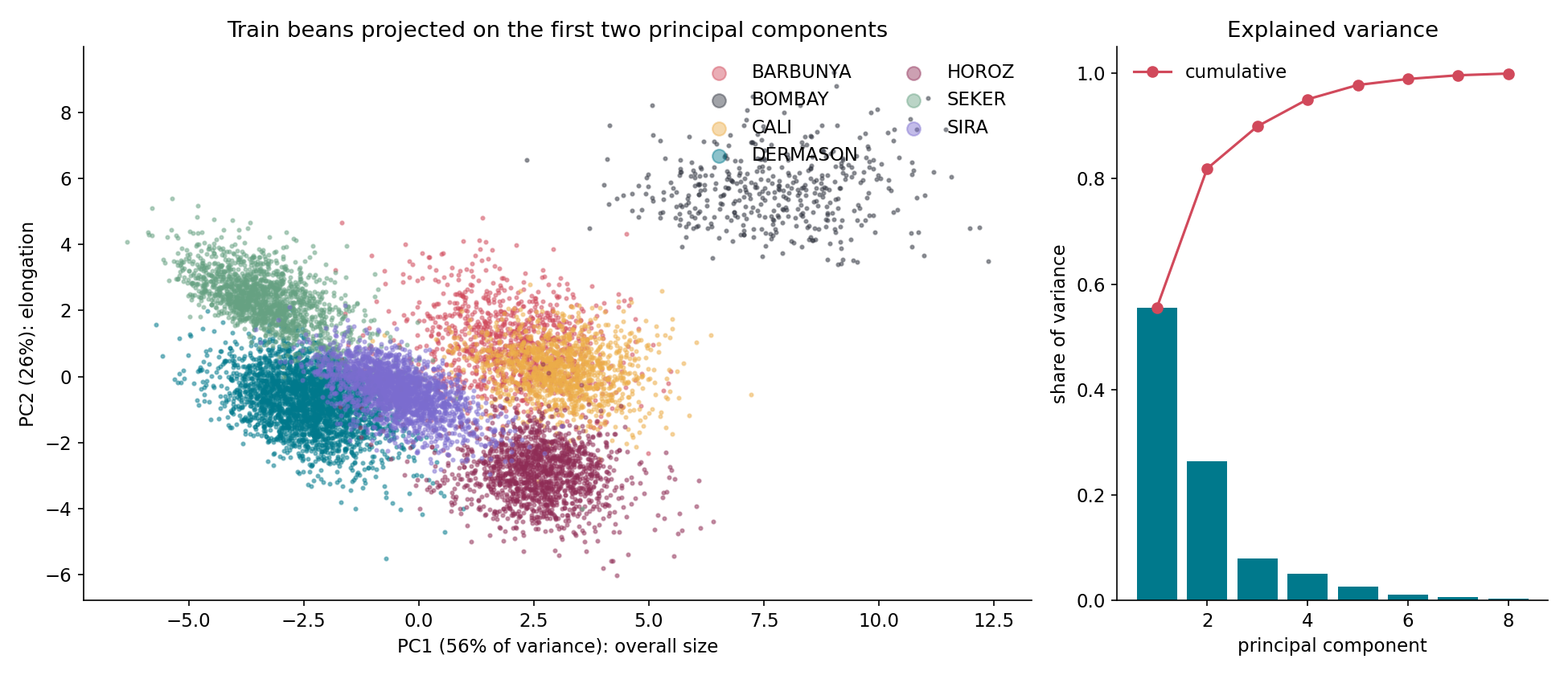
PCA projection of the training beans and explained variance

The first component explains 55.5 % of the variance, the first two 81.9 % and the first three 89.9 %. PC1 loads on the axis lengths, perimeter and diameter, so it measures size. PC2 loads on the minor axis, ShapeFactor1, aspect ratio and compactness, so it measures elongation. In this plane:

Bombay is far away on its own: these beans are huge, more than five times the area of a Dermason.
Horoz (long, thin) sits low on PC2 and Seker (round) sits high, so both separate well.
Dermason and Sira overlap heavily: they are small beans of similar shape that differ mostly in size, and their size ranges overlap.
Barbunya and Cali overlap too: both are large, and they differ in a subtle way (Cali is a bit more elongated).

These two overlapping pairs will turn out to be exactly the confusions that every model makes.

A first baseline

The statement asks for a shallow tree first. With max_depth=3, a tree has at most 8 leaves for 7 classes, so it should just about be able to name every variety. The surprise is in the results:

tree, depth 3	accuracy	macro F1	classes never predicted
criterion = gini	0.770	0.594	Barbunya and Bombay
criterion = entropy	0.800	0.741	Barbunya

Accuracy is a respectable 77 %, but the gini tree never predicts Bombay, the most separable variety of all. The reason is that gini's impurity, $1-\sum_c p_c^2$ , mostly rewards splits that clean up the large classes, so carving off 4 % of beans into their own leaf is worth little to it. Entropy, $-\sum_c p_c\log p_c$ , is a log measure: it gives more weight to rare classes, because creating a pure leaf removes a $p\log p$ term that is relatively large. For a shallow tree under macro F1, this difference is enormous (+15 points). It also makes shallow gini trees unstable: depending on the split, a class may or may not get a leaf, and the CV macro F1 at depth 4 swings with a standard deviation of 0.065.

The key idea

A decision tree only ever asks "is feature $j$ at most $t$ ?". That has three consequences, and together they settle every question in the statement.

Trees do not care about scale or about monotone transformations. Replacing $x_j$ by $a x_j + b$ , by $\log x_j$ or by $x_j^2$ (for positive values) leaves the ordering of the beans unchanged, so the tree can make exactly the same splits. We checked this directly: standardising the features or taking their logarithm gives exactly the same tree, with test macro F1 0.9171 in both cases, and ShapeFactor3 (which equals Compactness²) is a perfect substitute for Compactness. So trees need neither standardisation nor PCA for scale reasons.
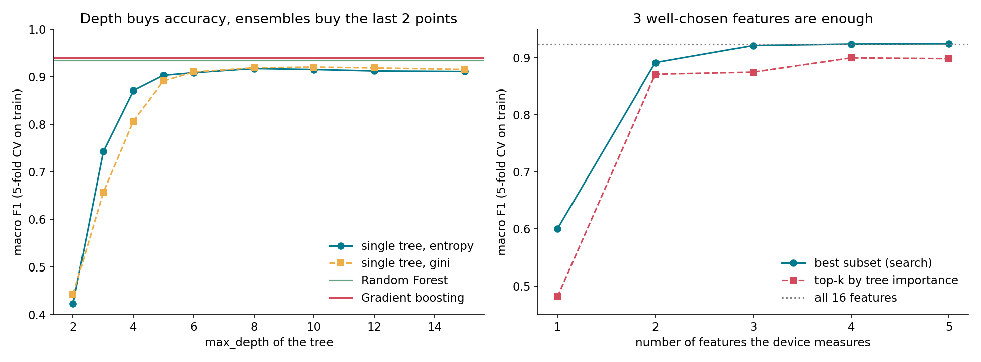
Feature importance is not feature selection. Because Compactness and ShapeFactor3 are interchangeable, the tree spreads its importance across copies of the same information. The top 3 features by impurity importance (ShapeFactor3, MajorAxisLength, ShapeFactor1) are two shape measures and one size measure, and two of them overlap in what they encode. They reach only 0.875 CV macro F1. An exhaustive search over all 560 three-feature subsets finds roundness + Compactness + ShapeFactor1 at 0.922, as good as all 16 features (0.924). Those three cover three different things: roundness compares area with perimeter, Compactness compares area with length, and ShapeFactor1 is the inverse thickness $L/A$ . And they need only three physical measurements: $A$ , $P$ and $L$ . That is the cheap machine the company wants.
One tree draws a staircase; an ensemble smooths it out. Every leaf is an axis-aligned box with a hard boundary. A bean sitting 0.03 standard deviations on the wrong side of a threshold is sent the wrong way, and nothing downstream can fix it. Averaging hundreds of trees, each built on different data (bagging, random forest) or correcting the previous trees' errors (boosting), turns the staircase into a smooth, almost oblique boundary. That is worth about 1.5 to 2 points of macro F1 here, and it also cuts the variance across splits in half. The price: there is no longer one path you can read.

The full solution

Step 1: preparation. Drop the 68 duplicates, then make a stratified 80/20 split (random_state=42). Use 5-fold stratified CV on the training part for every choice.

Step 2: tune a single tree. We searched over the criterion, max_depth from 6 to unlimited, and min_samples_leaf from 1 to 40, by CV. The winner is gini, max_depth=10, min_samples_leaf=10 (CV F1 0.924, test 0.917, 185 leaves). The left panel below shows the usual picture: performance rises steeply up to depth 5 or 6, then plateaus. An unrestricted tree slightly overfits (test F1 0.910), and constraining the leaf size helps more than limiting the depth.

Macro F1 against depth, and against number of features

Step 3: a readable tree to explain things. A 185-leaf tree is not something you can read. For interpretation we use a second tree with entropy, depth 4 and at least 20 beans per leaf: 16 leaves, test F1 0.877, and every variety has a leaf.

The readable depth-4 tree

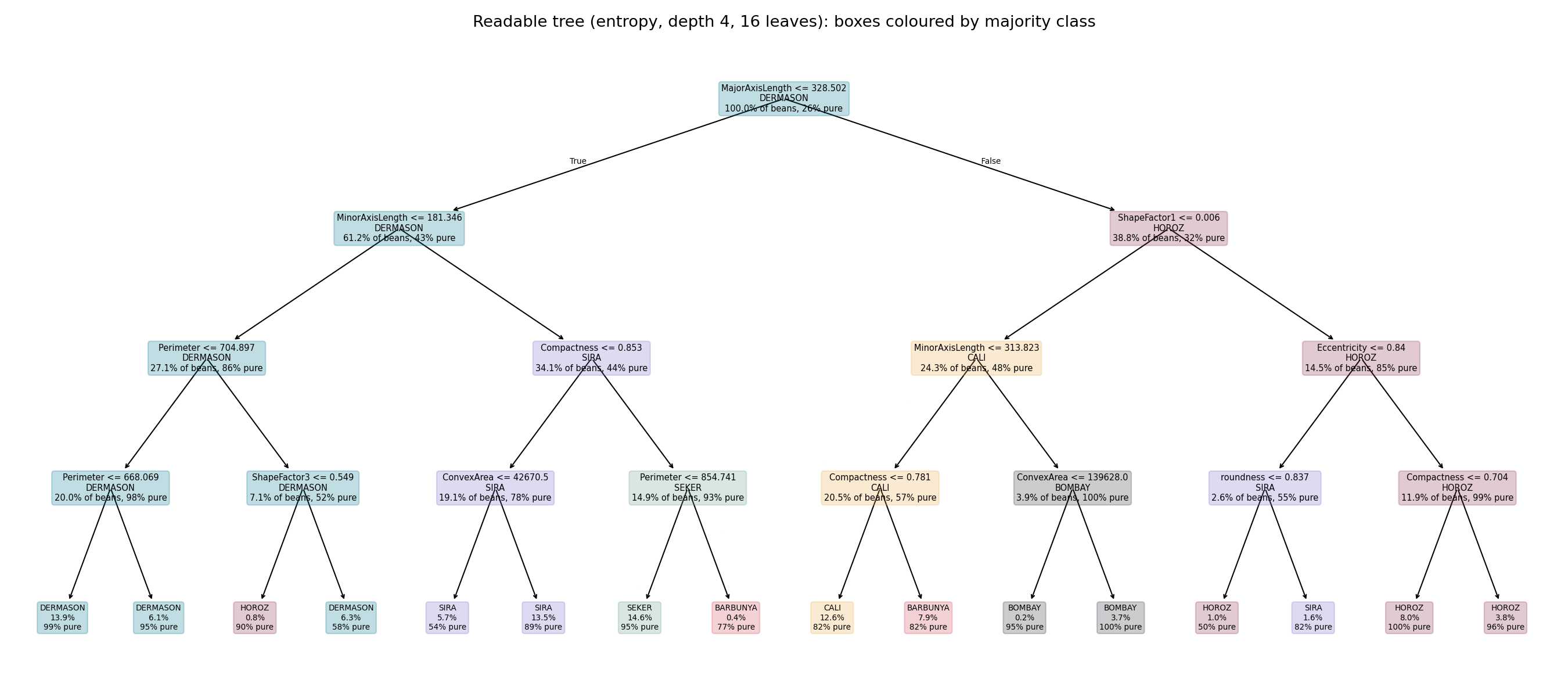
Its root asks one question, "is the major axis at most 328.5 pixels?", and that splits the beans into small ones (Dermason, Seker, Sira) and large ones (Barbunya, Bombay, Cali, Horoz). Here are the most useful rules, with support and purity measured on the training set:

#	rule	variety	beans	correct
1	$L \le 328.5$ , $l \le 181.3$ , $P \le 668$	Dermason	1506	99 %
2	$L \le 328.5$ , $l > 181.3$ , Compactness $> 0.853$ , $P \le 855$	Seker	1579	95 %
3	$L \le 328.5$ , $l > 181.3$ , Compactness $\le 0.853$ , ConvexArea $> 42\,670$	Sira	1458	89 %
4	$L > 328.5$ , ShapeFactor1 $> 0.00609$ , Eccentricity $> 0.840$ , Compactness $\le 0.704$	Horoz	869	100 %
5	$L > 328.5$ , ShapeFactor1 $\le 0.00609$ , $l > 313.8$ , ConvexArea $> 139\,628$	Bombay	399	100 %
6	$L > 328.5$ , ShapeFactor1 $\le 0.00609$ , $l \le 313.8$ , then Compactness $\le 0.781$ / $> 0.781$	Cali / Barbunya	1363 / 853	82 % / 82 %

In plain words: a small, thin bean is a Dermason. A small bean that is thick and nearly round (compactness above 0.85) is a Seker. A long bean with a very high eccentricity is a Horoz. A bean whose short axis alone exceeds 314 pixels is a Bombay. Rule 6 is the most telling one: Cali and Barbunya share the same box, and one compactness threshold is all that separates them, at only 82 % purity. The PCA plot already showed that these two overlap.

Step 4: dissecting three mistakes. For each misclassified bean, we follow its path and, at every node, look at the share of its true variety among the training beans that reach that node. The "wrong turn" is the node where the bean goes into the branch that holds less of its own variety than the other branch.

Bean 13211, a Dermason predicted as Sira. It passes $L = 268 \le 328.5$ , then hits $l = 184.9 > 181.3$ . That is only 0.08 standard deviations above the threshold, but Dermason drops from 43 % of the node to 8 % on that side. The bean is a slightly chubby Dermason, and from then on it lives among Siras.
Bean 7761, a Sira predicted as Dermason. It is the mirror case: its minor axis $l = 171.1$ falls 0.23 std below 181.3, so it ends up in the "thin, small" branch where Siras are only 10 %.
Bean 2257, a Barbunya predicted as Horoz. ShapeFactor1 is 0.006117 against a threshold of 0.006088, a gap of 0.03 std. That one hair of difference sends it to the long-bean side, where Barbunyas make up 2 %.

The pattern is always the same: the error is made at one node, by a bean sitting right on a threshold, and it involves exactly the pairs PCA showed as overlapping (Dermason and Sira, Barbunya and Cali, plus large-versus-elongated). Revealingly, the tuned 185-leaf tree and the boosted ensemble both classify all three beans correctly. Boosting gives bean 13211 a probability of 0.65 for Dermason against 0.34 for Sira, which is a fair description of a borderline case.

Step 5: ensembles. We trained three ensembles of trees: bagging (200 unpruned trees), a random forest (500 trees, random feature subsets at each split) and gradient boosting (HistGradientBoostingClassifier, learning rate 0.05, 300 rounds of depth-6 trees, L2 regularisation of 1). To measure stability, we refit each model on 10 different random 80/20 splits:

model	macro F1, mean over 10 splits	standard deviation
readable tree (depth 4)	0.869	0.0062
tuned tree	0.922	0.0044
random forest	0.933	0.0026
gradient boosting	0.938	0.0023

Ensembles are better and steadier, which is what the bias-variance view predicts. One deep tree has low bias but high variance: it changes a lot when the data changes. Averaging $B$ trees whose errors are only partly correlated (correlation $\rho$ , variance $\sigma^2$ each) gives variance $\rho\sigma^2 + \frac{1-\rho}{B}\sigma^2$ . The random forest lowers $\rho$ by forcing the trees to look at random features. Boosting instead reduces bias, step by step, by fitting each new tree to the errors of the previous ones. Interpretability is the price: 300 trees of 64 leaves cannot be read as rules. You are left with global tools (feature importance, partial dependence) and per-bean probabilities.

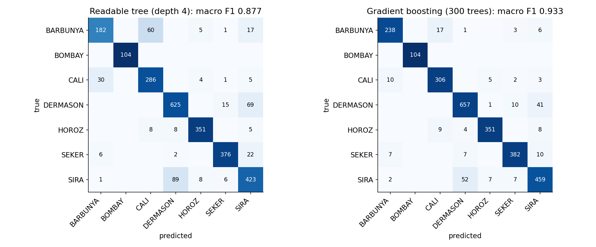
Confusion matrices of the readable tree and of gradient boosting

The confusion matrices tell the same story. Bombay is perfect in both. The readable tree's big errors are Barbunya predicted as Cali (60 beans) and Sira and Dermason mixed up (89 + 69 beans). Boosting divides the Barbunya/Cali errors by about 3, but Sira/Dermason stays the hard core (52 + 41 beans). Sira has the lowest per-class F1 (0.87) and Bombay the highest (1.00). These beans overlap in shape space, so no model built on silhouettes will fully separate them.

Step 6: PCA versus original features.

features	tuned tree	random forest
original 16	0.917	0.930
PCA, 2 components	0.859	0.852
PCA, 3 components	0.865	0.877
PCA, 5 components	0.909	0.924
PCA, all 16 components	0.916	0.932

(test macro F1)

Keeping 2 or 3 components throws away information that matters: the last 10 % of the variance contains much of what separates Dermason from Sira. The scatter plot is wonderful for seeing the classes, but it is a poor input for the classifier. Keeping all 16 components is a pure rotation and loses no information. The forest gains 0.2 points, which is within the split-to-split noise (std 0.0026), while the single tree gains nothing. In principle a rotation can help, because an oblique boundary in the original axes may become axis-aligned along a principal component, but here the gain is too small to measure. Meanwhile interpretability collapses: a split such as "PC2 ≤ 0.4" means a weighted mix of 16 features. Verdict: PCA is a visualisation tool here. Trees do not need it, and they read better without it.

Step 7: the cheap sorting machine. The right panel of the tradeoffs figure shows the best subset of $k$ features, found by exhaustive search for $k \le 3$ and by greedy extension for $k = 4, 5$ , all scored by CV on the training data only.

1 feature (EquivDiameter, i.e. size): 0.60. Size alone separates only Bombay and the small-versus-large groups.
2 features (Perimeter + ShapeFactor2): 0.89, a size measure plus a shape measure.
3 features (roundness, Compactness, ShapeFactor1): 0.922 CV, test macro F1 0.914 against 0.917 with all 16, a loss of 0.3 points. Accuracy goes from 0.904 to 0.903.
4 or 5 features: 0.924, no further gain.

Answers to the statement: three features, which need only three raw measurements (area, perimeter and length), are enough for sensible sorting. The tree loses less than half a point of macro F1, and about 1.9 points compared with the best ensemble on all features (0.933). A cheaper camera and simpler software are clearly worth it. The point you must not miss: picking the "3 most important features" from the full tree's importance ranking gives 0.880 on test, a full 3.4 points worse than a proper subset search, because importance is shared between redundant copies of the same information.

Results

All numbers are on our held-out 20 % split (2 709 beans). The official test labels are private.

approach	accuracy	macro F1
tree depth 3, gini (never predicts 2 classes)	0.770	0.594
tree depth 3, entropy	0.800	0.741
readable tree, depth 4, entropy (16 leaves)	0.866	0.877
unrestricted tree (overfits)	0.895	0.910
tuned tree: gini, depth 10, min leaf 10	0.904	0.917
tuned tree on standardised or log features (no change, as predicted)	0.904	0.917
tuned tree on 2 / 3 PCA components	0.859 / 0.861	0.859 / 0.865
tuned tree, 3 features chosen by importance	0.873	0.880
tuned tree, 3 searched features (cheap machine)	0.903	0.914
bagging, 200 trees	0.917	0.929
random forest, 500 trees	0.918	0.930
random forest on 16 PCA components	0.923	0.932
gradient boosting (final model)	0.922	0.933
gradient boosting on raw + PCA features	0.924	0.934
for reference, not a tree: RBF SVM on standardised features	0.924	0.935
for reference: soft vote of boosting + SVM	0.926	0.937

The final tree-based model, gradient boosting, reaches 0.933 macro F1 (92.2 % accuracy) on held-out data. Under the original paper's 10-fold protocol it reaches 93.0 % accuracy, matching the published reference of about 93 %. The extra tweaks (PCA features added to boosting, voting with an SVM) gain a few tenths of a point, which is within the noise. The problem is saturated by the Sira/Dermason overlap, not by the model.

What to remember

Read the metric before the model. Macro F1 gives the rarest class the same weight as the largest one. A shallow gini tree with 77 % accuracy scored 0.59 because it ignored Bombay. Check which classes your model never predicts.
Trees ask only "is $x_j \le t$ ?". So they ignore scaling and any monotone transformation, and they need neither standardisation nor PCA. PCA belongs in the plotting step, not in front of a tree.
Importance is not selection. With correlated features, importance spreads across copies of the same information. To choose a small set of features, search subsets with cross-validation, and think in terms of the physical measurements each feature needs (here 3 measurements give 16 features for free).
Single trees make errors at a threshold; ensembles soften the thresholds. That gives about 2 points of F1 and half the variance across splits, at the cost of readable rules. Keep a small tree for explaining and an ensemble for predicting.
Clean before you split. Exact duplicates leak between train and test. Here they were all from one class, which would have quietly inflated that class's score.

Full code (solution.py)

"""
Slovak AI Olympiad 2026, Task 1: recognising dry bean varieties with explainable tree models.

Data: UCI Dry Bean dataset (13 611 beans, 7 varieties, 16 shape features), downloaded from
https://archive.ics.uci.edu/static/public/602/dry+bean+dataset.zip and unzipped next to this file
(expects DryBeanDataset/Dry_Bean_Dataset.xlsx under DATA_DIR).

The official judge split is private, so everything is evaluated on our own stratified 80/20 split
(random_state=42). All model choices are made by 5-fold cross-validation on the 80 % train part;
the 20 % test part is touched only for the final numbers. Main metric: macro F1.

Run:  python solution.py   (about 3 minutes on a laptop CPU; figures go to ./figures)
"""
import itertools, os
import numpy as np, pandas as pd
import matplotlib; matplotlib.use("Agg")
import matplotlib.pyplot as plt
from joblib import Parallel, delayed
from sklearn.model_selection import train_test_split, StratifiedKFold, cross_val_score
from sklearn.preprocessing import StandardScaler
from sklearn.decomposition import PCA
from sklearn.pipeline import make_pipeline
from sklearn.tree import DecisionTreeClassifier, plot_tree
from sklearn.ensemble import RandomForestClassifier, BaggingClassifier, HistGradientBoostingClassifier
from sklearn.svm import SVC
from sklearn.metrics import accuracy_score, f1_score, confusion_matrix

DATA_DIR = os.environ.get("DATA_DIR", "work")
FIG = "figures"; os.makedirs(FIG, exist_ok=True)
plt.rcParams.update({"font.size": 11, "axes.spines.top": False, "axes.spines.right": False})
COLORS = dict(BARBUNYA="#d1495b", BOMBAY="#30343f", CALI="#edae49", DERMASON="#00798c",
              HOROZ="#8f2d56", SEKER="#66a182", SIRA="#7b6ccf")

# ---------------------------------------------------------------- 1. Data preparation
df = pd.read_excel(f"{DATA_DIR}/DryBeanDataset/Dry_Bean_Dataset.xlsx")
print("shape", df.shape, "| missing values:", int(df.isna().sum().sum()), "| duplicated rows:", int(df.duplicated().sum()))
print(df["Class"].value_counts().to_string())
# Sanity checks: the 16 features are formulas of a few raw measurements, verify them.
A, Pm, L, l = df.Area, df.Perimeter, df.MajorAxisLength, df.MinorAxisLength
checks = {"AspectRation = L/l": df.AspectRation - L / l,
          "roundness = 4 pi A / P^2": df.roundness - 4 * np.pi * A / Pm**2,
          "ShapeFactor1 = L/A": df.ShapeFactor1 - L / A,
          "ShapeFactor2 = A/L^3": df.ShapeFactor2 - A / L**3,
          "ShapeFactor3 = Compactness^2": df.ShapeFactor3 - df.Compactness**2,
          "ShapeFactor4 = A/(pi L l/4)": df.ShapeFactor4 - A / (np.pi * L * l / 4)}
for k, v in checks.items():
    print(f"  {k:30s} max |error| = {np.abs(v).max():.1e}")
# The 68 duplicated rows (all HOROZ) would leak between train and test: drop them.
df = df.drop_duplicates().reset_index(drop=True)
X, y = df.drop(columns="Class"), df["Class"]
FEATS = list(X.columns)
Xtr, Xte, ytr, yte = train_test_split(X, y, test_size=0.2, stratify=y, random_state=42)
CV = StratifiedKFold(5, shuffle=True, random_state=0)

def cv_f1(model, cols=FEATS):
    return cross_val_score(model, Xtr[cols], ytr, cv=CV, scoring="f1_macro", n_jobs=-1).mean()

RESULTS = []
def evaluate(name, model, cols=FEATS):
    """Fit on train, score on held-out test; store and print accuracy + macro F1."""
    model.fit(Xtr[cols], ytr); p = model.predict(Xte[cols])
    r = dict(model=name, acc=accuracy_score(yte, p), f1=f1_score(yte, p, average="macro"))
    RESULTS.append(r); print(f"  {name:42s} acc={r['acc']:.4f}  macroF1={r['f1']:.4f}")
    return model, p

# ---------------------------------------------------------------- 2. Correlations and PCA
corr = X.corr().abs()
pairs = sorted(((corr.iloc[i, j], FEATS[i], FEATS[j]) for i in range(16) for j in range(i + 1, 16)), reverse=True)
print("most correlated pairs:", [(a, b, round(c, 3)) for c, a, b in pairs[:6]])
scaler = StandardScaler().fit(Xtr)                      # PCA needs standardisation (Area ~ 1e5, ShapeFactor2 ~ 1e-3)
pca = PCA().fit(scaler.transform(Xtr))
evr = pca.explained_variance_ratio_
print("explained variance PC1..PC4:", np.round(evr[:4], 3), "cumulative:", np.round(np.cumsum(evr)[:4], 3))
Z = pca.transform(scaler.transform(Xtr))
fig, ax = plt.subplots(1, 2, figsize=(13, 5.6), gridspec_kw=dict(width_ratios=[2.2, 1]))
for c in sorted(COLORS):
    m = (ytr == c).values
    ax[0].scatter(Z[m, 0], Z[m, 1], s=4, alpha=.45, color=COLORS[c], label=c, rasterized=True)
ax[0].set_xlabel(f"PC1 ({evr[0]:.0%} of variance): overall size"); ax[0].set_ylabel(f"PC2 ({evr[1]:.0%}): elongation")
ax[0].legend(markerscale=4, frameon=False, ncol=2, loc="upper right"); ax[0].set_title("Train beans projected on the first two principal components")
ax[1].bar(range(1, 9), evr[:8], color="#00798c"); ax[1].plot(range(1, 9), np.cumsum(evr[:8]), "o-", color="#d1495b", label="cumulative")
ax[1].set_xlabel("principal component"); ax[1].set_ylabel("share of variance"); ax[1].set_ylim(0, 1.05)
ax[1].legend(frameon=False); ax[1].set_title("Explained variance")
fig.tight_layout(); fig.savefig(f"{FIG}/pca.png", dpi=150); plt.close(fig)
load = pd.DataFrame(pca.components_[:2].T, index=FEATS, columns=["PC1", "PC2"])
print("PC1 top loadings:", load.PC1.abs().sort_values(ascending=False).index[:4].tolist(),
      "| PC2 top loadings:", load.PC2.abs().sort_values(ascending=False).index[:4].tolist())

# ---------------------------------------------------------------- 3. Decision trees
print("\nDecision trees (CV macro F1 on train)")
for d in [2, 3, 4, 5, 6, 8, 10, 12, None]:
    print(f"  max_depth={d}: gini {cv_f1(DecisionTreeClassifier(max_depth=d, random_state=0)):.4f}"
          f" | entropy {cv_f1(DecisionTreeClassifier(max_depth=d, criterion='entropy', random_state=0)):.4f}")
grid = list(itertools.product(["gini", "entropy"], [6, 8, 10, 12, None], [1, 5, 10, 20, 40]))
scores = [cv_f1(DecisionTreeClassifier(criterion=c, max_depth=d, min_samples_leaf=s, random_state=0)) for c, d, s in grid]
crit, depth, leaf = grid[int(np.argmax(scores))]
print(f"  best by CV: criterion={crit}, max_depth={depth}, min_samples_leaf={leaf}, CV F1={max(scores):.4f}")
print("Held-out test")
evaluate("Tree depth 3 (gini)", DecisionTreeClassifier(max_depth=3, random_state=0))
evaluate("Tree depth 3 (entropy)", DecisionTreeClassifier(max_depth=3, criterion="entropy", random_state=0))
small, p_small = evaluate("Readable tree depth 4 (entropy, leaf>=20)",
                          DecisionTreeClassifier(max_depth=4, criterion="entropy", min_samples_leaf=20, random_state=0))
big, p_big = evaluate(f"Tuned tree ({crit}, depth {depth}, leaf {leaf})",
                      DecisionTreeClassifier(criterion=crit, max_depth=depth, min_samples_leaf=leaf, random_state=0))
evaluate("Unrestricted tree", DecisionTreeClassifier(random_state=0))
print(f"  readable tree: {small.get_n_leaves()} leaves | tuned tree: {big.get_n_leaves()} leaves, depth {big.get_depth()}")
fig, ax = plt.subplots(figsize=(18, 8))
plot_tree(small, feature_names=FEATS, class_names=small.classes_, impurity=False,
          proportion=True, precision=3, fontsize=7, ax=ax)
for t in ax.texts:
    if t.get_text().count("<=") == 0: t.set_fontsize(6.5)
for t in ax.texts:  # shorten each box to "split / class (share of beans, purity)" and colour it by class
    lines = t.get_text().split("\n")
    if len(lines) < 3: continue
    cls = lines[-1].split("class = ")[-1]; share = lines[-3].split("= ")[-1]
    purity = max(float(v) for v in lines[-2].split("[")[1].rstrip("]").split(","))
    head = lines[0] + "\n" if len(lines) == 4 else ""
    t.set_text(f"{head}{cls}\n{share} of beans, {purity:.0%} pure" if head else f"{cls}\n{share}\n{purity:.0%} pure")
    if cls in COLORS: t.set_bbox(dict(boxstyle="round", fc=COLORS[cls], alpha=.25, ec=COLORS[cls]))
ax.set_title("Readable tree (entropy, depth 4, 16 leaves): boxes coloured by majority class")
fig.tight_layout(); fig.savefig(f"{FIG}/tree.png", dpi=150); plt.close(fig)

# ---------------------------------------------------------------- 4. Rules and errors
def leaf_rules(tree, X_, y_):
    """Every leaf as a rule: conditions on the path, predicted class, support and purity on train."""
    t = tree.tree_; rules = []
    def rec(node, conds):
        if t.children_left[node] == -1:
            idx = tree.apply(X_) == node
            cls = tree.classes_[np.argmax(t.value[node])]
            rules.append((" and ".join(conds), cls, int(idx.sum()), float((y_[idx] == cls).mean())))
            return
        f, thr = FEATS[t.feature[node]], t.threshold[node]
        rec(t.children_left[node], conds + [f"{f} <= {thr:.4g}"])
        rec(t.children_right[node], conds + [f"{f} > {thr:.4g}"])
    rec(0, []); return sorted(rules, key=lambda r: -r[2] * r[3])
print("\nRules from the readable tree (support on train, purity):")
for cond, cls, n, pur in leaf_rules(small, Xtr, ytr)[:8]:
    print(f"  IF {cond}  THEN {cls}   [{n} beans, {pur:.0%} correct]")

def explain(tree, x, true):
    """Walk the path of one bean; flag the node where the branch taken holds less of the true class."""
    t = tree.tree_; node = 0; Xa = Xtr.values; ya = ytr.values; inside = np.ones(len(Xa), bool)
    sd = Xtr.std()
    while t.children_left[node] != -1:
        f, thr = t.feature[node], t.threshold[node]
        go_left = x[f] <= thr
        left = inside & (Xa[:, f] <= thr); right = inside & ~(Xa[:, f] <= thr)
        share = lambda m: (ya[m] == true).mean() if m.any() else 0
        taken, other = (left, right) if go_left else (right, left)
        flag = "  <== wrong turn" if share(other) > share(taken) else ""
        print(f"     {FEATS[f]} = {x[f]:.4g} {'<=' if go_left else '>'} {thr:.4g}"
              f"  (gap {abs(x[f] - thr) / sd.iloc[f]:.2f} std; {true} share {share(inside):.0%} -> {share(taken):.0%}){flag}")
        inside = taken; node = t.children_left[node] if go_left else t.children_right[node]
wrong = np.where(p_small != yte.values)[0]
pairs_seen = set(); print("\nMisclassified test beans (readable tree):")
for i in wrong:
    pair = (yte.values[i], p_small[i])
    if pair in pairs_seen or len(pairs_seen) >= 3: continue
    pairs_seen.add(pair); print(f"  bean #{Xte.index[i]}: true {pair[0]}, predicted {pair[1]}")
    explain(small, Xte.values[i], pair[0])

# ---------------------------------------------------------------- 5. Ensembles and stability
print("\nEnsembles (held-out test)")
hgb = lambda s=0: HistGradientBoostingClassifier(learning_rate=0.05, max_iter=300, max_depth=6, l2_regularization=1.0, random_state=s)
evaluate("Bagging (200 full trees)", BaggingClassifier(DecisionTreeClassifier(), n_estimators=200, n_jobs=-1, random_state=0))
rf, _ = evaluate("Random Forest (500 trees)", RandomForestClassifier(500, n_jobs=-1, random_state=0))
gb, p_gb = evaluate("Gradient Boosting (HistGB, 300 trees)", hgb())
evaluate("Reference, not a tree: RBF SVM", make_pipeline(StandardScaler(), SVC(C=10)))
print("Stability over 10 different random 80/20 splits (macro F1 mean +- std):")
stab = {"Tree depth 4": lambda s: DecisionTreeClassifier(max_depth=4, criterion="entropy", min_samples_leaf=20, random_state=s),
        "Tuned tree": lambda s: DecisionTreeClassifier(criterion=crit, max_depth=depth, min_samples_leaf=leaf, random_state=s),
        "Random Forest": lambda s: RandomForestClassifier(500, n_jobs=-1, random_state=s), "HistGB": hgb}
for name, make in stab.items():
    f = []
    for s in range(10):
        a, b, ya, yb = train_test_split(X, y, test_size=0.2, stratify=y, random_state=100 + s)
        f.append(f1_score(yb, make(s).fit(a, ya).predict(b), average="macro"))
    print(f"  {name:15s} {np.mean(f):.4f} +- {np.std(f):.4f}  (min {np.min(f):.4f})")

labels = sorted(COLORS)
fig, ax = plt.subplots(1, 2, figsize=(13, 5.4))
for a, p, title in [(ax[0], p_small, "Readable tree (depth 4)"), (ax[1], p_gb, "Gradient boosting (300 trees)")]:
    cm = confusion_matrix(yte, p, labels=labels); cmn = cm / cm.sum(1, keepdims=True)
    a.imshow(cmn, cmap="Blues", vmin=0, vmax=1)
    for i in range(7):
        for j in range(7):
            if cm[i, j]: a.text(j, i, cm[i, j], ha="center", va="center", fontsize=9, color="white" if cmn[i, j] > .6 else "black")
    a.set_xticks(range(7), labels, rotation=45, ha="right"); a.set_yticks(range(7), labels)
    a.set_xlabel("predicted"); a.set_ylabel("true"); a.set_title(f"{title}: macro F1 {f1_score(yte, p, average='macro'):.3f}")
fig.tight_layout(); fig.savefig(f"{FIG}/confusion.png", dpi=150); plt.close(fig)

# ---------------------------------------------------------------- 6. PCA vs original features
print("\nPCA components vs original features (held-out test)")
tuned = lambda: DecisionTreeClassifier(criterion=crit, max_depth=depth, min_samples_leaf=leaf, random_state=0)
for k in [2, 3, 5, 16]:
    evaluate(f"PCA {k} comps + tuned tree", make_pipeline(StandardScaler(), PCA(k), tuned()))
    evaluate(f"PCA {k} comps + Random Forest", make_pipeline(StandardScaler(), PCA(k), RandomForestClassifier(500, n_jobs=-1, random_state=0)))
evaluate("Tuned tree on standardised features", make_pipeline(StandardScaler(), tuned()))  # identical: trees ignore scale

# ---------------------------------------------------------------- 7. A cheap device: 3 to 5 features
print("\nFeature subsets for the tuned tree (CV macro F1 on train)")
imp = pd.Series(big.feature_importances_, FEATS).sort_values(ascending=False)
print("  impurity importances:", imp.round(3).head(6).to_dict())
curve = {"importance": [], "search": []}
best_subsets = {}
for k in range(1, 6):
    top = list(imp.index[:k]); curve["importance"].append(cv_f1(tuned(), top))
    if k <= 3:   # exhaustive search over all C(16,k) subsets
        combos = [list(c) for c in itertools.combinations(FEATS, k)]
    else:        # greedy: extend the best (k-1)-subset by one feature
        combos = [best_subsets[k - 1] + [f] for f in FEATS if f not in best_subsets[k - 1]]
    s = Parallel(n_jobs=-1)(delayed(lambda c: cross_val_score(tuned(), Xtr[c], ytr, cv=CV, scoring="f1_macro").mean())(c) for c in combos)
    best_subsets[k] = combos[int(np.argmax(s))]; curve["search"].append(max(s))
    print(f"  k={k}: top-k by importance {curve['importance'][-1]:.4f} | best subset {best_subsets[k]} {max(s):.4f}")
all_cv = cv_f1(tuned())
evaluate("Tuned tree on 3 features " + "+".join(best_subsets[3]), tuned(), best_subsets[3])
evaluate("HistGB on the same 3 features", hgb(), best_subsets[3])
evaluate("Tuned tree on top-3 by importance", tuned(), list(imp.index[:3]))
fig, ax = plt.subplots(1, 2, figsize=(13, 4.8))
ds = [2, 3, 4, 5, 6, 8, 10, 12, 15]
ax[0].plot(ds, [cv_f1(DecisionTreeClassifier(max_depth=d, criterion="entropy", random_state=0)) for d in ds], "o-", color="#00798c", label="single tree, entropy")
ax[0].plot(ds, [cv_f1(DecisionTreeClassifier(max_depth=d, random_state=0)) for d in ds], "s--", color="#edae49", label="single tree, gini")
for name, v, c in [("Random Forest", cv_f1(RandomForestClassifier(300, n_jobs=-1, random_state=0)), "#66a182"), ("Gradient boosting", cv_f1(hgb()), "#d1495b")]:
    ax[0].axhline(v, color=c, lw=1.5, label=name)
ax[0].set_xlabel("max_depth of the tree"); ax[0].set_ylabel("macro F1 (5-fold CV on train)")
ax[0].set_ylim(0.4, 1); ax[0].legend(frameon=False, loc="lower right"); ax[0].set_title("Depth buys accuracy, ensembles buy the last 2 points")
ks = range(1, 6)
ax[1].plot(ks, curve["search"], "o-", color="#00798c", label="best subset (search)")
ax[1].plot(ks, curve["importance"], "s--", color="#d1495b", label="top-k by tree importance")
ax[1].axhline(all_cv, color="gray", ls=":", label="all 16 features")
ax[1].set_xticks(list(ks)); ax[1].set_xlabel("number of features the device measures"); ax[1].set_ylabel("macro F1 (5-fold CV on train)")
ax[1].set_ylim(0.45, 0.95); ax[1].legend(frameon=False, loc="lower right"); ax[1].set_title("3 well-chosen features are enough")
fig.tight_layout(); fig.savefig(f"{FIG}/tradeoffs.png", dpi=150); plt.close(fig)

print("\nSummary (held-out 20 % test, official test labels are private)")
print(pd.DataFrame(RESULTS).drop_duplicates("model").round(4).to_string(index=False))