IOAI Training: Learn AI by solving problems

The problem in brief

You are handed a PyTorch implementation of a convolutional sentence classifier "based on" Kim (2014), Convolutional Neural Networks for Sentence Classification, trained on MR: 10 662 one-sentence movie-review snippets labelled positive or negative. It reaches less than 60 % accuracy, while the paper reports 76.1 % for its simplest variant. Task 1: read the paper and fix four deviations (dropout, optimiser, pooling, filter sizes and batch size), explaining the optimiser change. Task 2: improve further with a component or architecture change of your choice (pretrained embeddings, recurrent networks or a Transformer), justify it and run it.

How you are scored

A selection test graded by the coaches: each step must be implemented and run, with the logs kept, and the written answers must be correct. The quantitative yardstick is test accuracy on the fixed split of the starter notebook (the first 80 % of each class for training, the next 10 % for validation, the last 10 % for test: 8 530 / 1 066 / 1 066 sentences), with the model chosen on validation accuracy:

\text{accuracy} = \frac{\#\{\text{test sentences classified correctly}\}}{1\,066}.

Targets from the paper (which uses 10-fold cross-validation, so numbers are comparable but not identical): 76.1 % for CNN-rand (random embeddings), 81.0 to 81.5 % with pretrained word2vec vectors.

First look at the data

Perfectly balanced classes (5 331 each): accuracy is a fair metric and 50 % is chance.
Sentences are short, 21 tokens on average, at most 59: a whole review fits in one window of a few dozen tokens.
Sentiment is carried by a few phrases ("a gorgeous, witty, seductive movie", "not worth the price"), wherever they appear in the sentence. That observation decides the pooling question below.
The training set is small (8 530 sentences) for learning 300-dimensional embeddings of 18 000 words from scratch: pretrained knowledge should matter a lot.

A first baseline

The starter, run as given (mean pooling, filters of width 2/3/4 with 50 maps, no dropout, plain SGD with the default learning rate $10^{-3}$ , batch 25, 50 epochs, words seen fewer than 5 times replaced by <unk>): 59.8 % test accuracy, 60.4 % on validation. Its training accuracy is still only 63 % after 50 epochs (figure below): the model is not overfitting, it is barely learning. That diagnosis already points at the optimiser.

The key idea

Task 1 is about matching the paper detail by detail, and each detail has a reason.

Step 1, dropout. Kim applies dropout with $p = 0.5$ on the penultimate layer: the vector of pooled filter outputs, just before the final linear layer. During training each of the 300 features is zeroed with probability 0.5, so the classifier cannot rely on one co-adapted detector. The paper also rescales and clips the output weights to an L2 norm of at most $s = 3$ (max-norm); we implement it too.

Step 2, the optimiser: Adadelta instead of plain SGD. SGD applies the same global step to every parameter, $\theta \leftarrow \theta - \eta\, g$ , and with $\eta = 10^{-3}$ that step is far too small here. Adadelta (Zeiler, 2012) keeps two running averages per parameter, of squared gradients and of squared updates, with decay $\rho = 0.95$ :

E[g^2]_t = \rho\, E[g^2]_{t-1} + (1-\rho)\, g_t^2, \qquad \Delta\theta_t = -\frac{\sqrt{E[\Delta\theta^2]_{t-1} + \varepsilon}}{\sqrt{E[g^2]_t + \varepsilon}}\; g_t, \qquad E[\Delta\theta^2]_t = \rho\, E[\Delta\theta^2]_{t-1} + (1-\rho)\, \Delta\theta_t^2 .

The differences that matter: (i) the step size is per parameter and adapts to the scale of its gradients, which is ideal for embeddings, where a rare word's row receives a gradient only a few times per epoch and still gets a meaningful update; (ii) the ratio of the two RMS terms has the units of the parameter itself, so there is no learning rate to tune (PyTorch's lr=1.0 is the paper's setting); (iii) it is robust to badly scaled gradients across layers. With it, training converges in a few epochs instead of crawling.

Step 3, pooling: max over time instead of mean. Each filter is a detector of one n-gram pattern; its activation along the sentence is high where the pattern occurs. Max pooling keeps the strongest occurrence, wherever it is, and ignores the length of the sentence. Mean pooling dilutes one decisive phrase among all the neutral positions, so "boring" in a 40-token sentence weighs four times less than in a 10-token one. For "is this pattern present?", max is the right summary.

Step 4, filters and batch. Widths 3, 4, 5 with 100 feature maps each (a 300-dimensional sentence vector) and mini-batches of 50.

Two further paper details turned out to matter as much as the four steps: the vocabulary keeps every training word (min_freq=1, the starter used 5), and random embeddings are drawn from $U[-0.25, 0.25]$ . With PyTorch's default $\mathcal{N}(0, 1)$ initialisation the same model reached only 68.5 %: Adadelta's first updates are tiny ( $\approx \sqrt{\varepsilon}/\text{RMS}(g)$ ), so vectors that start 7 times too large barely move. Matching the paper's initial scale brought us to 76 %.

Task 2: give the model knowledge it cannot learn from 8 530 sentences.

Pretrained word vectors (our first choice, the paper's CNN-non-static): initialise the embedding layer with GloVe 6B 300-d vectors, trained on 6 billion tokens of Wikipedia and news, and keep fine-tuning them. "Superb" and "terrific" then start close together even if only one appears in training. Only the embedding initialisation changes; 16 159 of our 18 064 words have a GloVe vector, the others stay random in $U[-0.25, 0.25]$ .
A pretrained Transformer (second choice): replace the whole CNN by DistilBERT, a 6-layer Transformer pretrained by masked language modelling, with a linear classifier on its [CLS] representation, fine-tuned end to end (AdamW, learning rate $2\cdot10^{-5}$ , linear warm-up and decay, 2 epochs). Self-attention reads the sentence in context, so it can handle negation and contrast ("not bad at all", "pretty but empty"), which a bag of local n-gram detectors misses.

The full solution

solution.py re-implements the notebook without the deprecated torchtext (the basic_english tokenizer is re-written in 10 lines) and runs every variant with the same data split:

class CNN(nn.Module):
    def forward(s, ids):
        x = s.emb(ids).permute(0, 2, 1)                         # (batch, 300, length)
        h = [torch.relu(conv(x)) for conv in s.convs]           # widths 3, 4, 5, 100 maps each
        h = [t.max(dim=-1).values for t in h]                   # Step 3: max over time
        return s.fc(s.drop(torch.cat(h, -1)))                   # Step 1: dropout 0.5 before fc

opt = torch.optim.Adadelta(model.parameters(), lr=1.0, rho=0.95, eps=1e-6)   # Step 2
# after each step: rescale rows of fc.weight to L2 norm <= 3 (paper's max-norm)

Sentences are padded to at least 5 tokens so that the widest filter always has a window. Every model keeps the epoch with the best validation accuracy, and the test set is evaluated once at the end. CNN runs use 2 seeds and report both.

Results

model	validation	test
starter as given (mean pooling, SGD $10^{-3}$ , no dropout)	0.604	0.598
Task 1 with PyTorch's default $\mathcal{N}(0,1)$ embedding init (failed attempt)	0.687	0.685
Task 1: Kim CNN-rand (seeds 0 / 1)	0.751 / 0.745	0.760 / 0.755
Task 2a: + GloVe 300-d, fine-tuned (seeds 0 / 1)	0.787 / 0.781	0.794 / 0.783
Task 2b: DistilBERT fine-tuned, 2 epochs	0.853	0.844

Task 1 reproduces the paper's 76.1 % almost exactly (mean 75.8 %). Pretrained word vectors add 3 points (paper: about 5 with word2vec); a pretrained Transformer adds another 5.6, for a total gain of 24.5 points over the starter. Fine-tuning DistilBERT took 9 minutes on a laptop GPU (Apple MPS).

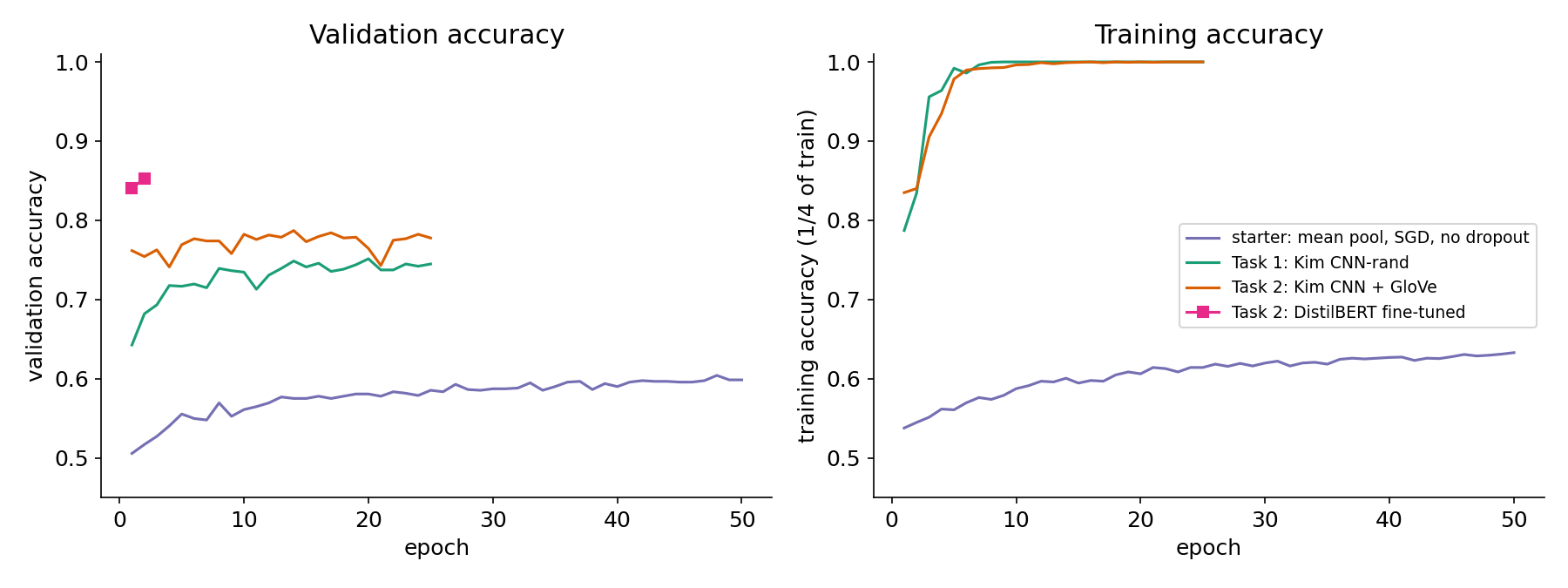
Validation and training accuracy per epoch. The starter crawls from 50 % to 60 % in 50 epochs; the Kim CNN reaches 100 % training accuracy within 10 epochs while validation plateaus around 74 to 75 %; with GloVe validation sits around 78 %; DistilBERT is at 84 to 85 % after one or two epochs.

The curves tell the story of the two tasks. The starter is under-fitting: wrong optimiser and step size, and mean pooling, which washes out the signal. The Kim CNN fits the training set perfectly in under 10 epochs and then overfits (validation stops improving while training reaches 100 %, despite dropout): it has learnt all it can from 8 530 sentences. Beyond that point the only lever is outside knowledge, which is exactly what pretrained embeddings and pretrained Transformers bring.

What to remember

Read the training curve before touching the model: low training accuracy means under-fitting (optimiser, learning rate, capacity, pooling); training at 100 % with validation stuck means over-fitting (regularisation, more data, pretraining).
Max pooling detects "is the pattern anywhere?"; mean pooling measures "how much of the sentence is the pattern?". Choose the summary that matches the question.
Adaptive optimisers (Adadelta, Adam) give each parameter its own step size, which matters most for sparse embedding gradients.
Reproducing a paper means reproducing all of it, including "minor" details such as initialisation scale and vocabulary thresholds; here the initialisation alone was worth 7 points.
Small datasets are won by transfer: pretrained word vectors help, a pretrained Transformer fine-tuned for two epochs helps much more.

"""Singapore IOAI 2024 selection test, NLP: Kim (2014) CNN for sentence classification on MR.

Data: rt-polaritydata.tar.gz (the file behind HF jeffnyman/rotten_tomatoes_reviews), split exactly as
that loader does: first 80 % of each class = train, next 10 % = validation, last 10 % = test.

  python solution.py starter    # the given model: mean pooling, plain SGD, no dropout (< 60 %)
  python solution.py kim        # Task 1: dropout 0.5, Adadelta, max-over-time pooling, 3/4/5 x 100, batch 50
  python solution.py glove      # Task 2a: same CNN, embeddings initialised with GloVe 6B-300d (fine-tuned)
  python solution.py bert       # Task 2b: fine-tune a pretrained Transformer (DistilBERT)
Files: work/rt-polaritydata/ (curl https://testerstories.com/files/ai_learn/rt-polaritydata.tar.gz | tar xz)
       work/glove300.pt = {"itos", "vectors"} built from the HF repo
       sentence-transformers/average_word_embeddings_glove.6B.300d (0_WordEmbeddings/model.safetensors
       + whitespacetokenizer_config.json "vocab"); DistilBERT via transformers.
Every run: 2 seeds (1 for the starter and BERT), model chosen on validation accuracy, test accuracy reported once at the end.
"""
import json, re, sys, time
import numpy as np, torch, torch.nn as nn

torch.set_num_threads(2)
DEV = torch.device("mps" if torch.backends.mps.is_available() else "cpu")
DATA = "work/rt-polaritydata/rt-polarity."

def load_split():
    pos = [l.decode("latin-1").strip() for l in open(DATA + "pos", "rb")]
    neg = [l.decode("latin-1").strip() for l in open(DATA + "neg", "rb")]
    i1, i2 = int(len(pos) * 0.8 + 0.5), int(len(pos) * 0.9 + 0.5)
    mk = lambda a, b: (pos[a:b] + neg[a:b], [1] * len(pos[a:b]) + [0] * len(neg[a:b]))
    return mk(0, i1), mk(i1, i2), mk(i2, None)

# torchtext "basic_english" tokenizer, re-implemented (torchtext is no longer maintained)
_PAT = [(r"\'", " '  "), (r"\"", ""), (r"\.", " . "), (r"<br \/>", " "), (r",", " , "), (r"\(", " ( "),
        (r"\)", " ) "), (r"\!", " ! "), (r"\?", " ? "), (r"\;", " "), (r"\:", " "), (r"\s+", " ")]
def tokenize(s):
    s = s.lower()
    for p, r in _PAT: s = re.sub(p, r, s)
    return s.split()[:256]

class CNN(nn.Module):
    def __init__(s, V, E, n_filters, sizes, pool="max", dropout=0.0, emb=None):
        super().__init__()
        s.emb = nn.Embedding(V, E, padding_idx=1)
        if emb is not None: s.emb.weight.data.copy_(emb)
        s.convs = nn.ModuleList([nn.Conv1d(E, n_filters, k) for k in sizes])
        s.pool, s.drop = pool, nn.Dropout(dropout)
        s.fc = nn.Linear(len(sizes) * n_filters, 2)
        for m in list(s.convs) + [s.fc]:
            (nn.init.kaiming_normal_(m.weight, nonlinearity="relu") if isinstance(m, nn.Conv1d)
             else nn.init.xavier_normal_(m.weight)); nn.init.zeros_(m.bias)
    def forward(s, ids):
        x = s.emb(ids).permute(0, 2, 1)
        h = [torch.relu(c(x)) for c in s.convs]
        # max-over-time keeps the strongest match of each n-gram detector, wherever it occurs;
        # the mean dilutes one decisive phrase ("not good") among all the neutral positions
        h = [t.max(-1).values if s.pool == "max" else t.mean(-1) for t in h]
        return s.fc(s.drop(torch.cat(h, -1)))      # dropout on the penultimate layer (paper, p = 0.5)

def batches(X, y, bs, shuffle, rng, minlen=5):
    idx = rng.permutation(len(X)) if shuffle else np.arange(len(X))
    for k in range(0, len(idx), bs):
        b = idx[k:k + bs]; L = max(minlen, max(len(X[i]) for i in b))   # pad to >= largest filter
        t = torch.ones(len(b), L, dtype=torch.long)
        for j, i in enumerate(b): t[j, :len(X[i])] = torch.tensor(X[i])
        yield t, torch.tensor([y[i] for i in b])

def accuracy(model, X, y):
    model.eval(); ok = 0
    with torch.no_grad():
        for t, l in batches(X, y, 200, False, None): ok += (model(t.to(DEV)).argmax(-1).cpu() == l).sum().item()
    return ok / len(y)

def run_cnn(mode, seed):
    (trT, trY), (vaT, vaY), (teT, teY) = load_split()
    trT, vaT, teT = [list(map(tokenize, S)) for S in (trT, vaT, teT)]
    cnt = {}
    for s in trT:
        for w in s: cnt[w] = cnt.get(w, 0) + 1
    min_freq = 5 if mode == "starter" else 1      # the paper keeps every training word
    itos = ["<unk>", "<pad>"] + sorted(w for w in cnt if cnt[w] >= min_freq)
    stoi = {w: i for i, w in enumerate(itos)}
    enc = lambda S: [[stoi.get(w, 0) for w in s] for s in S]
    trX, vaX, teX = enc(trT), enc(vaT), enc(teT)
    torch.manual_seed(seed); rng = np.random.default_rng(seed)
    # paper: random vectors drawn from U[-0.25, 0.25] (PyTorch's default N(0, 1) is 7x larger, and
    # Adadelta's tiny first steps then barely move them)
    emb = None if mode == "starter" else torch.empty(len(itos), 300).uniform_(-0.25, 0.25)
    if mode == "glove":                               # Task 2a: pretrained vectors
        g = torch.load("work/glove300.pt")            # {"itos": [...], "vectors": Tensor}
        gi = {w: i for i, w in enumerate(g["itos"])}
        hit = 0
        for w, i in stoi.items():
            if w in gi: emb[i] = g["vectors"][gi[w]]; hit += 1
        print(f"GloVe covers {hit}/{len(itos)} words")
    if mode == "starter":
        model = CNN(len(itos), 300, 50, [2, 3, 4], pool="mean", dropout=0.0)
        opt = torch.optim.SGD(model.parameters(), lr=1e-3, weight_decay=0.0025); bs = 25
    else:
        if emb is not None: emb[1] = 0                # padding vector
        model = CNN(len(itos), 300, 100, [3, 4, 5], pool="max", dropout=0.5, emb=emb)
        opt = torch.optim.Adadelta(model.parameters(), lr=1.0, rho=0.95, eps=1e-6); bs = 50
    model.to(DEV)                                     # in place: the optimizer keeps the same Parameters
    crit, best, hist = nn.CrossEntropyLoss(), (-1, None), []
    for ep in range(50 if mode == "starter" else 25):
        model.train()
        for t, l in batches(trX, trY, bs, True, rng):
            opt.zero_grad(); loss = crit(model(t.to(DEV)), l.to(DEV)); loss.backward(); opt.step()
            if mode != "starter":                     # paper: l2-norm constraint s = 3 on the output weights
                with torch.no_grad():
                    n = model.fc.weight.norm(dim=1, keepdim=True).clamp(min=3.0)
                    model.fc.weight.mul_(3.0 / n)
        va = accuracy(model, vaX, vaY); hist.append((accuracy(model, trX[::4], trY[::4]), va)); print(ep, hist[-1], flush=True)
        if va > best[0]: best = (va, {k: v.clone() for k, v in model.state_dict().items()})
    model.load_state_dict(best[1])
    return {"val": best[0], "test": accuracy(model, teX, teY), "hist": hist}

def run_bert(seed, name="distilbert-base-uncased", epochs=2):
    from transformers import AutoTokenizer, AutoModelForSequenceClassification, get_linear_schedule_with_warmup
    (trT, trY), (vaT, vaY), (teT, teY) = load_split()
    dev = torch.device("mps" if torch.backends.mps.is_available() else "cpu")
    tok = AutoTokenizer.from_pretrained(name); torch.manual_seed(seed); rng = np.random.default_rng(seed)
    model = AutoModelForSequenceClassification.from_pretrained(name, num_labels=2).to(dev)
    opt = torch.optim.AdamW(model.parameters(), lr=2e-5, weight_decay=0.01)
    steps = epochs * (len(trT) + 31) // 32
    sch = get_linear_schedule_with_warmup(opt, int(0.1 * steps), steps)
    def acc(T, Y):
        model.eval(); ok = 0
        with torch.no_grad():
            for k in range(0, len(T), 128):
                b = tok(T[k:k + 128], padding=True, truncation=True, max_length=64, return_tensors="pt").to(dev)
                ok += (model(**b).logits.argmax(-1).cpu() == torch.tensor(Y[k:k + 128])).sum().item()
        return ok / len(Y)
    best, hist = (-1, None), []
    for ep in range(epochs):
        model.train(); idx = rng.permutation(len(trT))
        for k in range(0, len(idx), 32):
            b = idx[k:k + 32]
            enc = tok([trT[i] for i in b], padding=True, truncation=True, max_length=64, return_tensors="pt").to(dev)
            out = model(**enc, labels=torch.tensor([trY[i] for i in b]).to(dev))
            opt.zero_grad(); out.loss.backward(); opt.step(); sch.step()
            if (k // 32) % 50 == 0: print("step", k // 32, round(out.loss.item(), 3), flush=True)
        va = acc(vaT, vaY); hist.append(va); print("epoch", ep, "val", va, flush=True)
        if va > best[0]: best = (va, {k: v.detach().cpu().clone() for k, v in model.state_dict().items()})
    model.load_state_dict(best[1])
    return {"val": best[0], "test": acc(teT, teY), "hist": hist}

if __name__ == "__main__":
    mode = sys.argv[1]; seeds = {"starter": [0], "bert": [0]}.get(mode, [0, 1])
    res = []
    for sd in seeds:
        t0 = time.time()
        r = run_bert(sd) if mode == "bert" else run_cnn(mode, sd)
        r["minutes"] = (time.time() - t0) / 60; res.append(r)
        print(mode, "seed", sd, "val %.4f test %.4f (%.1f min)" % (r["val"], r["test"], r["minutes"]), flush=True)
    print(mode, "mean test %.4f +- %.4f" % (np.mean([r["test"] for r in res]), np.std([r["test"] for r in res])))
    json.dump(res, open(f"work/res_{mode}.json", "w"))

Deep Learning for NLP: CNN sentence classification