IOAI Final Selection Test (Computer Vision)

The problem in brief

This camp test has two parts built on CIFAR-10 (60,000 color images of 32x32 pixels, 10 classes) and a ResNet-18 given in the notebook. Task 1 compares ways of using pretrained knowledge: finetune an ImageNet ResNet-18, train the same network from scratch, classify with CLIP without any training (zero-shot), improve CLIP with a prompt ensemble, then learn the class "text" vectors on the training set. Task 2 builds a deliberately imbalanced training set (100 % of airplanes and cars down to 2 % of ships and trucks) and asks you to diagnose and fix the damage: per-class precision and recall, balanced sampling, loss weighting, and a free final push. The CIFAR-10 test set and its labels are public, so every number below is measured on the official 10,000 test images. The notebook comes from a third-party repository (github.com/teodora-dimitrova/Singapore-Team-Selection); the copy there already contains one contestant's answers, which we did not use.

How you are scored

Each question has marks for code, accuracy and short reports, with the expected accuracy written next to it (Q1.1 about 88 %, Q1.2 about 55 %, Q1.3 about 90 %, Q1.4 about 91 %, Q2.1 about 69 %). Two questions have a formula:

• Q1.5 (10 marks for accuracy): $\max\{\min\{\tfrac{acc - 91}{96}, 1\} \times 10,\ \tfrac{i}{N} \times 10\}$, where $i/N$ is your relative rank. Taken literally, the fraction can never exceed $5/96$; the intended formula is almost certainly $\tfrac{acc-91}{96-91}$: zero marks at 91 %, full marks at 96 %.
• Q2.5 (10 marks): $\min\{\tfrac{acc-85}{95}, 1\} \times 10$, read the same way as $\tfrac{acc-85}{95-85}$: full marks at 95 %.

First look at the setup

Before running anything, read the notebook's ResNet carefully, because it is not torchvision's.

• The stem has stride 1 and no max-pool. A 32x32 image stays 32x32 through layer1, and the final feature map is 4x4. This is the usual CIFAR adaptation, and it makes the network about 16 times more expensive than torchvision's ResNet-18 on the same tiny input. The ImageNet 7x7 filters are still loaded, they just slide with a different stride.
• The BatchNorm layers inside the blocks have track_running_stats=False. They always normalise with the statistics of the current batch, even in eval() mode. So the test accuracy depends on the test batches (100 images in file order): harmless here, but a trap if you ever predict one image at a time.
• Loading pretrained weights with strict=False hides mismatches. Our check is to print the missing keys: they must be only fc.weight and fc.bias. The running-mean buffers of the untracked BatchNorms show up as "unexpected" keys and are rightly ignored.

We downloaded CIFAR-10 from the Hugging Face mirror uoft-cs/cifar10 (identical images) and loaded all pretrained weights from safetensors files.

Task 1: what pretraining buys you

Q1.1 and Q1.2, finetuning against training from scratch. With the notebook's settings (SGD, learning rate 0.01, momentum 0.9, weight decay $5\times10^{-4}$, batch 128, crop and flip augmentation, one epoch), the ImageNet-initialised network reaches 89.7 % and the randomly initialised one 57.6 %. The pretrained filters already detect edges, textures and object parts, so one pass over CIFAR-10 is enough to adapt them; from scratch, one epoch only starts learning those filters. The price of finetuning: you inherit the pretrained architecture (here its 7x7 stem, designed for 224-pixel images), its input normalisation and its biases, and the gain shrinks when the target domain is far from ImageNet (medical scans, spectrograms).

Q1.3, CLIP zero-shot. CLIP embeds images and sentences in the same 512-dimensional space. To classify, embed the sentence "a photo of a {class}." for the 10 classes, normalise everything, and pick the class whose text vector has the largest cosine similarity with the image. With ViT-B/32 on the full test set: 88.3 %, with no training at all.

One technical lesson cost us 3 points before we found it. OpenAI trained CLIP with the QuickGELU activation, $x\,\sigma(1.702\,x)$. Loading the same weights into a model that uses the exact GELU (open_clip's ViT-B-32 instead of ViT-B-32-quickgelu) runs without any error and gives 85.1 %. Weights only make sense with the exact architecture they were trained with.

Q1.4, prompt ensembling. Embed the class name in the 7 templates of the CLIP paper ("itap of a {}.", "a bad photo of the {}.", "a origami {}." and so on), normalise each embedding, average them per class and renormalise. Accuracy rises to 90.0 % (88.3 % with one prompt, 87.4 % with the bare class name). Why it works: each sentence's embedding is the class concept plus noise that depends on the wording ("origami" pulls towards paper, "video game" towards renders). Averaging over different wordings cancels that wording-specific noise and keeps the common direction, exactly as averaging several noisy measurements reduces the variance. It also covers more of the visual styles in which the class can appear. The notebook's own hint of "~90 %" and "~91 %" comes from evaluating on about 100 random images, where one image is worth a full percentage point.

Q1.5, learning the class vectors. Now we keep the image encoder frozen and make the 10 class vectors trainable. Computing CLIP features for every image once (batches of 250 on the GPU, 4 minutes for the training set) turns the problem into training a tiny model on 50,000 vectors of dimension 512:

$$\text{logit}_c(x) = s \cdot \frac{f(x)}{\lVert f(x) \rVert} \cdot \frac{w_c}{\lVert w_c \rVert},$$

where $f(x)$ is the frozen image feature, $w_c$ the learnable vector of class $c$, initialised with the prompt-ensemble embedding, and $s = e^{\tau}$ a learnable temperature initialised at 100 and capped there, as in CLIP's own code. AdamW (learning rate $10^{-3}$, cosine schedule, 30 epochs, batch 256). For augmentation in feature space we also computed the features of the mirrored images and trained on both views, then averaged both views at test time.

• On a 5,000-image validation split carved out of the training set: 95.2 % (95.5 % with the flip average).
• On the test set: 95.2 % with flip averaging (95.1 % without), so about 8.5 of the 10 accuracy marks with the intended formula.

Two observations for the report. The initialisation mostly buys speed: a random initialisation ends at 94.9 % on validation, but the text-initialised model is already at 90 % before the first step. And the learned vectors move far from the text: their cosine with the initial text embedding ends around 0.5, because the best classifier in image space is not the text direction, only a good starting point. Reaching 96 % with a frozen ViT-B/32 would need a stronger image encoder or finetuning the image tower.

Task 2: an imbalanced training set

Q2.1. Keeping each image of class $i$ with probability keep_ratio[i] (we fixed the random seed) leaves 18,763 images, from 5,000 airplanes and cars to 108 ships and 91 trucks. Finetuning for 3 epochs (about the same number of steps as one epoch on the full set) gives 69.9 % on the balanced test set.

Q2.2, precision and recall per class. For each class, count true positives, false positives (predicted $c$, truly another class) and false negatives (truly $c$, predicted another class); then precision $= TP/(TP+FP)$ and recall $= TP/(TP+FN)$.

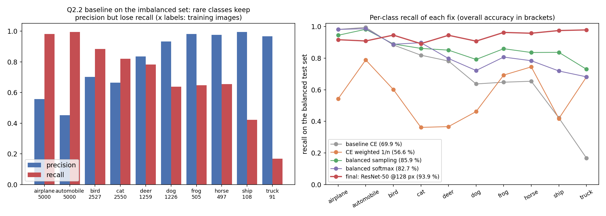
The pattern is the signature of a prior learned from data. The frequent classes have high recall and low precision (airplane recall 0.98 but precision 0.56, automobile 1.00 and 0.45): the model says "airplane" or "car" whenever it hesitates, so it catches all of them and many intruders. The rare classes have the opposite profile (truck recall 0.17 with precision 0.97, ship 0.42 and 1.00): the model only says "truck" when it is very sure, so what it says is right but it misses most trucks. The confusion matrix shows where they go: 763 of the 1,000 test trucks are predicted as automobiles, and ships go to airplanes (332) and cars (224), the visually closest frequent classes. The reason is the cross-entropy itself. Minimising the average loss over a training set with 55 cars per truck learns $p(\text{class} \mid x)$ under the training prior; on a balanced test set, the decision boundaries sit too far into the territory of the rare classes.

Q2.3, balanced sampling. Draw a class uniformly, then an image of that class uniformly: every batch now looks balanced. Accuracy jumps to 85.9 % and the truck recall from 0.17 to 0.73. The cost: the 91 trucks are each seen about 20 times per epoch, so the model risks memorising them (augmentation helps).

Q2.4, weighting the loss. We tried three weightings of the cross-entropy (normalised to average 1 over classes) and one logit correction:

weighting	test accuracy
none (Q2.1)	69.9 %
$w_c \propto 1/n_c$	56.6 %
$w_c \propto 1/\sqrt{n_c}$	74.3 %
effective number, $w_c \propto (1-\beta)/(1-\beta^{n_c})$, $\beta = 0.999$	76.4 %
balanced softmax: train on $z_c + \log \pi_c$	82.7 %

Plain inverse frequency is the worst: each truck weighs 55 times a car, so a single truck in a batch dominates the gradient, the effective learning rate on rare classes explodes and training becomes noisy (the frequent classes' recall collapses to 0.4 to 0.5). The softer weightings help a little. The best option is not a weight at all. Balanced softmax (logit adjustment) adds $\log \pi_c$, the log of the training frequency, to each logit during training only. The network then learns logits $z_c$ such that $\operatorname{softmax}(z + \log\pi)$ fits the imbalanced training data; since Bayes' rule says $p_{\text{train}}(c\mid x) \propto p(x\mid c)\,\pi_c$, the learned $z_c$ estimates $\log p(x \mid c)$ up to a constant, which is exactly the right score for a balanced test set. It corrects the prior without changing how often each image is seen.

Q2.5, the final push. Training longer helps everyone: the notebook's ResNet-18 with balanced softmax, label smoothing 0.1, a one-cycle schedule (10 epochs, peak learning rate 0.05) and flip averaging at test reaches 88.3 %. The big step, though, comes from using the pretrained network the way it was pretrained. An ImageNet ResNet-50 expects objects of 100 pixels or more; we upsample each 32x32 image to 128x128 on the GPU, keep torchvision's stem (stride 2 and max-pool), normalise with ImageNet's mean and standard deviation, and finetune for 6 epochs (SGD, one-cycle up to 0.02, batch 64, weight decay $10^{-4}$, balanced softmax and label smoothing), then average each test image with its mirror. Result: 93.9 % (93.3 % without the flip), about 8.9 of the 10 marks. Every class has a recall of at least 0.89, trucks 0.98 and ships 0.97: with good features, 100 examples per class are enough, as long as the prior is corrected. This run took 12 minutes on a laptop GPU; a couple more epochs or 160-pixel inputs would likely close the remaining gap to 95 %.

Results

All on the official CIFAR-10 test set (10,000 images).

question	approach	accuracy	notebook's hint
Q1.1	ImageNet ResNet-18 finetuned, 1 epoch	89.7 %	~88 %
Q1.2	same network from scratch, 1 epoch	57.6 %	~55 %
Q1.3	CLIP ViT-B/32 zero-shot, "a photo of a {}."	88.3 %	~90 %
	same with GELU instead of QuickGELU (bug)	85.1 %
Q1.4	7-prompt ensemble	90.0 %	~91 %
Q1.5	learnable class vectors on frozen CLIP features, flip views	95.2 %	full marks at 96 %
Q2.1	imbalanced set, 3 epochs	69.9 %	~69 %
Q2.3	balanced sampling	85.9 %
Q2.4	best weighting: balanced softmax	82.7 %
Q2.5	ResNet-18, balanced softmax + LS, 10 epochs, flip TTA	88.3 %
Q2.5	ResNet-50 at 128 px, balanced softmax + LS, 6 epochs, flip TTA	93.9 %	full marks at 95 %

What to remember

• Pretraining is the biggest lever, if you respect it. One epoch of finetuning beats training from scratch by 32 points, and feeding the ImageNet ResNet-50 images at a resolution close to what it was trained on was worth more than every imbalance trick together.
• Weights come with an exact architecture. QuickGELU against GELU, a stem's stride, BatchNorm statistics, input normalisation: a mismatch rarely crashes, it silently costs accuracy. Check missing keys and sanity-check a known number.
• Prompt ensembling is variance reduction. Averaging normalised text embeddings over several wordings cancels the wording-specific noise, and the result is an excellent initialisation for a learned linear head.
• Imbalance shows up as a precision/recall asymmetry. Frequent classes get high recall and low precision, rare classes the reverse; look per class, never only at overall accuracy.
• Correct the prior rather than reweighting blindly. Inverse-frequency weights make training unstable; balanced sampling or balanced softmax ($z_c + \log\pi_c$ during training) fix the boundary with far less damage.