IOAI Training: Learn AI by solving problems

The problem in brief

Each old photo is given only as a 384-number embedding (the output of some image encoder), and you must guess the year it was taken, between 1900 and 2026. There are 1626 labelled photos and 3022 test photos (twice as many as the training set). The twist: for every photo you may give two guesses, and only the better one counts. The program submitted to Kattis simply prints the 3022 pairs of guesses.

How you are scored

For photo $i$ with true year $y_i$ and guesses $g_{i,1}, g_{i,2}$ , the error is the smaller of the two squared errors, and $E$ is its mean:

e_i = \min\big((g_{i,1}-y_i)^2,\ (g_{i,2}-y_i)^2\big), \qquad E = \frac{1}{N}\sum_i e_i , \qquad \text{Score} = 100\cdot\max\Big(0,\min\Big(1,\frac{300-E}{300-100}\Big)\Big).

So $E = 300$ gives 0 points and $E = 100$ gives 100. The test years are private; we evaluate with 5-fold cross-validation on the training set.

First look at the data

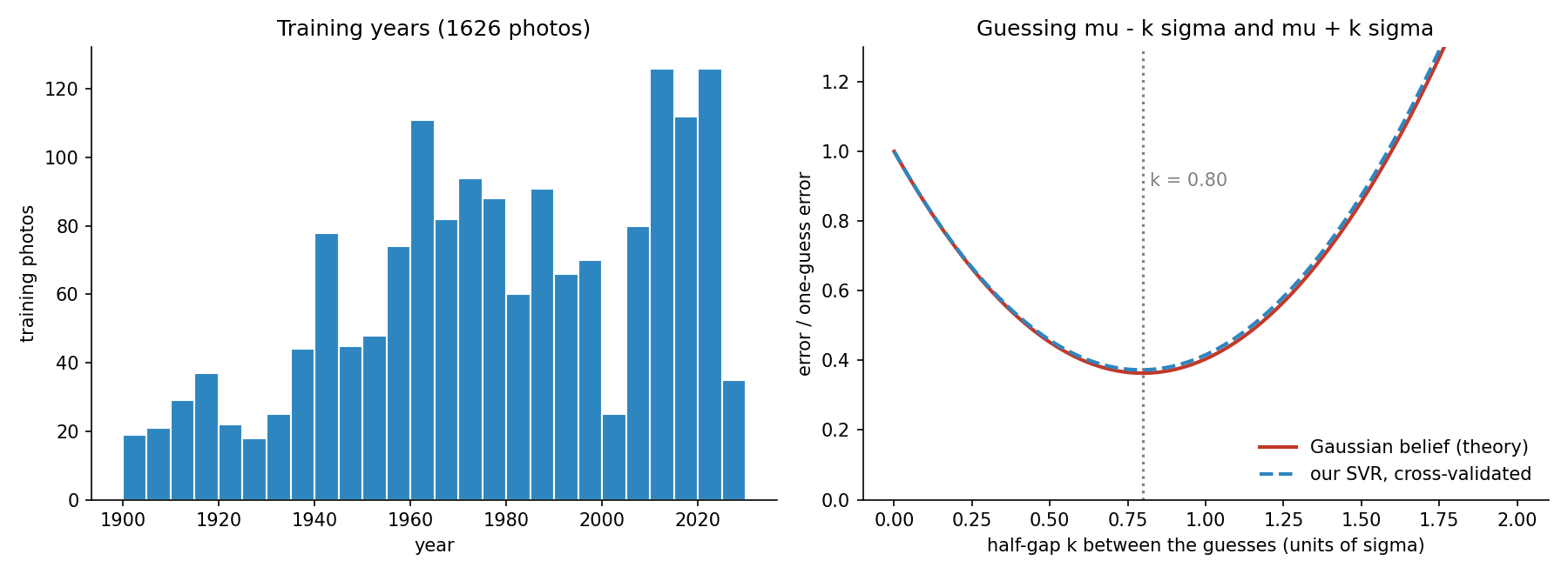
The years spread over the whole century (standard deviation 33 years), with peaks in the 1960s and the 2010s and a hole around 2000 (left panel of the figure). Predicting the mean year gives a squared error of 1078, far from the 300 needed for even one point.
The embeddings all have nearly the same length (about 47 to 48), so their direction carries the information: normalising them to unit length and using a cosine-like kernel is natural.
1626 examples in 384 dimensions is little data: strongly regularised or kernel models are the right tools, deep networks overfit.

A first baseline

Ridge regression on the embeddings, one guess repeated twice: squared error 471, score 0. A support vector regressor (RBF kernel on normalised embeddings) does better, 389, still 0 points. Even a good single guess cannot reach the scoring range: the photos are genuinely ambiguous, a 1970s street scene and a 1980s one look alike. The two-guess rule is where the points are.

The key idea

Two guesses turn a regression into a small quantisation problem. Suppose your belief about the year of a photo is $Y \sim \mathcal{N}(\mu, \sigma^2)$ . With one guess, the best is $\mu$ and the expected error is $\sigma^2$ . With two guesses $\mu - k\sigma$ and $\mu + k\sigma$ (symmetric by symmetry of the belief), write $Y = \mu + \sigma Z$ :

\mathbb{E}\big[\min((Z-k)^2, (Z+k)^2)\big]\,\sigma^2 = \mathbb{E}\big[(|Z|-k)^2\big]\,\sigma^2 = \Big(1 - 2k\sqrt{2/\pi} + k^2\Big)\sigma^2 ,

because the closer guess is always the one on the same side as $Z$ , and $\mathbb{E}|Z| = \sqrt{2/\pi}$ . Minimising over $k$ gives

k^* = \sqrt{2/\pi} \approx 0.80, \qquad \text{expected error} = \Big(1 - \frac{2}{\pi}\Big)\sigma^2 \approx 0.36\,\sigma^2 .

Two well-placed guesses cut the error by a factor of 2.75. One guess bets on "a bit earlier than my estimate", the other on "a bit later". Our cross-validated SVR follows this theory almost exactly (right panel): its error falls from 389 to 145 at $k = 0.8$ . (This is the same mathematics as the best 1-bit quantiser of a Gaussian signal, or k-means with $k = 2$ on the belief distribution.)

Left: histogram of training years from 1900 to 2026, with peaks around 1960 and 2015 and few photos around 2000. Right: error of the guess pair mu minus k sigma and mu plus k sigma, divided by the one-guess error, as a function of k; the Gaussian theory and our cross-validated SVR overlap, with a minimum of about 0.36 at k = 0.8.

Two refinements follow from the same formula.

A better centre $\mu$ lowers $\sigma^2$ and therefore everything else. We average the SVR with the mean of a predictive distribution from a multinomial logistic regression over 5-year bins: two different models, whose average has a squared error of 375 instead of 389.
A per-photo spread. $\sigma$ is not the same for every photo: some are easy to date, others not. We train a second SVR to predict the absolute error $|y - \mu|$ from the embedding (on out-of-fold residuals, so it learns real errors, not training-set errors) and place the guesses at $\mu \pm K\,\hat\sigma(x)$ . The predicted spread is a noisy proxy (correlation 0.25 with the actual error), so the best $K$ is not exactly 0.8: cross-validation picks $K = 1.2$ . Finally we clip the guesses to $[1900, 2026]$ : a guess outside the possible range is wasted.

The full solution

Normalise the embeddings to unit length for the SVRs; standardise them for the logistic regression.
Centre: $\mu(x) = \frac{1}{2}\big(\text{SVR}(x) + \sum_b P(b\mid x)\, m_b\big)$ , with $m_b$ the middle of 5-year bin $b$ .
Spread: out-of-fold residuals $|y-\mu|$ inside the training set, then an SVR to predict them, floored at 2 years.
Guesses: $\text{clip}(\mu \mp 1.2\,\hat\sigma)$ , rounded to integers.

mu, s = fit_predict(X, y, Xt)                         # centre and per-photo spread
g = np.clip(np.c_[mu - 1.2 * s, mu + 1.2 * s], 1900, 2026)

The evaluation is a nested cross-validation: in each outer fold, the spread model is trained on residuals computed by an inner cross-validation of the training part only.

Results

5-fold cross-validation on the 1626 training photos (the official test labels are private):

approach	one-guess squared error	two-guess error $E$	score
mean year, twice	1078	1078	0
ridge, same guess twice	471	471	0
ridge, $\mu \pm 0.8\sigma$	471	180	60.1
k-nearest neighbours (cosine, $k=20$ ), $\mu \pm 0.8\sigma$	618	215	42.4
SVR ( $C=300$ ), $\mu \pm 0.8\sigma$	389	145	77.4
logistic regression on 5-year bins, best pair under its predicted distribution		162	69.1
MLP with two outputs trained on the min-loss directly (failed idea)		159	70.5
SVR + logistic centre, $\mu \pm 0.8\sigma$	375	148	76.2
same centre, per-photo spread $\mu \pm 1.2\,\hat\sigma(x)$ (final)	375	139.5	80.3

Training a network directly on the "min of two squared errors" loss is elegant but did worse than the simple rule: with 1600 examples it overfits, and it must learn from scratch what the Gaussian argument gives for free. Our $K = 1.2$ was chosen on the same cross-validation it is reported on, so the final number may be slightly optimistic (the choice between $K = 1.0$ and $1.2$ changes it by only 1.6).

What to remember

Read the metric for hidden freedoms. "Two guesses, the best counts" changes the optimal answer from the mean to a pair around it.
With two guesses under a Gaussian belief, use $\mu \pm 0.8\sigma$ : the expected squared error drops from $\sigma^2$ to $0.36\sigma^2$ . The derivation takes three lines and is worth more than any model tuning.
Predict your own uncertainty. A model of $|y - \mu|$ trained on out-of-fold residuals lets you widen the pair for hard photos and tighten it for easy ones.
Small data, high dimension: kernel methods and regularised linear models beat neural networks here.
Use the valid range: clipping the guesses to the possible years is free accuracy.

"""SAIO "Time Guessing": two year guesses per photo embedding, only the better one counts.

  1. Centre = average of two regressors on the 384-d embeddings:
       a) SVR (RBF kernel, C = 300) on L2-normalised embeddings,
       b) the mean of a predictive distribution from multinomial logistic regression
          over 5-year bins (C = 0.1 on standardised features).
  2. Spread = expected size of the error for THIS photo: a second SVR trained to
     predict |y - centre| (out-of-fold residuals), floored at 2 years.
  3. Guesses = centre -/+ K * spread, clipped to [1900, 2026].
     For a Gaussian belief N(mu, s^2) the best pair is mu -/+ 0.80 s, cutting the
     expected squared error from s^2 to 0.36 s^2; K is tuned by cross-validation
     because the predicted spread is only a rough proxy for s.
Run: python solution.py   (expects train.json, test.json; prints CV error, writes answer.txt)
"""
import json
import numpy as np
from sklearn.linear_model import LogisticRegression
from sklearn.model_selection import KFold
from sklearn.preprocessing import StandardScaler
from sklearn.svm import SVR

K_SPREAD = 1.2
tr = json.load(open("train.json")); te = json.load(open("test.json"))
X = np.array([d["embedding"] for d in tr], np.float32); y = np.array([float(d["year"]) for d in tr])
Xt = np.array([d["embedding"] for d in te], np.float32)
BINS = np.arange(1900, 2030, 5)
GRID = np.arange(1900, 2027, 1.0)


def unit(A):
    return A / np.linalg.norm(A, axis=1, keepdims=True)


def centre(Xa, ya, Xb):
    svr = SVR(C=300, epsilon=1).fit(unit(Xa), ya).predict(unit(Xb))
    yb = np.clip(((ya - 1900) // 5).astype(int), 0, len(BINS) - 1)
    sc = StandardScaler().fit(Xa)
    lr = LogisticRegression(C=0.1, max_iter=2000).fit(sc.transform(Xa), yb)
    P = lr.predict_proba(sc.transform(Xb))                 # distribution over 5-year bins
    mid = BINS[lr.classes_] + 2.0                          # bin centres
    return (svr + P @ mid) / 2


def fit_predict(Xa, ya, Xb, seed=0):
    """Centre for Xb and a spread model trained on out-of-fold residuals of Xa."""
    oof = np.zeros(len(ya))
    for a, b in KFold(5, shuffle=True, random_state=seed).split(Xa):
        oof[b] = centre(Xa[a], ya[a], Xa[b])
    spread = SVR(C=10, epsilon=1).fit(unit(Xa), np.abs(ya - oof)).predict(unit(Xb))
    return centre(Xa, ya, Xb), np.maximum(spread, 2.0)


def guesses(mu, s, k=K_SPREAD):
    return np.clip(np.c_[mu - k * s, mu + k * s], 1900, 2026)


def err(g, yy):
    return np.minimum((g[:, 0] - yy) ** 2, (g[:, 1] - yy) ** 2).mean()


if __name__ == "__main__":
    # honest-ish evaluation: outer 5-fold CV, the spread model is nested inside each fold
    mu, s = np.zeros(len(y)), np.zeros(len(y))
    for a, b in KFold(5, shuffle=True, random_state=42).split(X):
        mu[b], s[b] = fit_predict(X[a], y[a], X[b])
    sg = np.sqrt(((mu - y) ** 2).mean())
    print(f"one guess (centre) MSE: {sg**2:.1f}")
    print(f"two guesses, constant spread 0.8*sigma: {err(guesses(mu, sg, 0.8), y):.1f}")
    for k in (1.0, 1.2, 1.4):
        E = err(guesses(mu, s, k), y)
        print(f"two guesses, per-photo spread, k={k}: {E:.1f} -> score {100*max(0,min(1,(300-E)/200)):.1f}")
    mu_t, s_t = fit_predict(X, y, Xt)
    g = np.rint(guesses(mu_t, s_t)).astype(int)
    open("answer.txt", "w").write("\n".join(f"{a} {b}" for a, b in g) + "\n")