IOAI Training: Learn AI by solving problems

The problem in brief

You are given 243 700 short user reviews (mostly of mobile apps) with their star rating, and 104 444 reviews without rating. You must predict the rating of each test review. No external data is allowed, and the only pretrained model you may use is bert-base-uncased, which the organisers' notebook downloads. Your Kattis submission simply prints one predicted rating per test review.

How you are scored

The metric is the mean squared error,

S = \frac{1}{n}\sum_{i=1}^{n} (X_i - Y_i)^2 ,

mapped linearly to points with $\text{baseline} = 3.5$ and $\text{best} = 0.5$ :

\text{Score} = \max\Big(0, \min\Big(100,\ 100\,\frac{3.5 - S}{3.5 - 0.5}\Big)\Big).

The final ranking uses 70 % of the test set, the visible leaderboard the other 30 %. Test ratings are private, so we hold out 40 000 random training reviews as a validation set and never touch it for training.

First look at the data

Ratings are very unbalanced: 59 % are 5 stars, 18 % are 1 star, the rest is spread over 2, 3 and 4 (with a few half stars). Predicting the training mean (3.9) already gives an MSE of 2.44 (35 points); predicting 3 everywhere gives 3.25.
Reviews are short: median 25 characters ("Good", "Great app!!", "Could be faster"), 90 % under 150 characters. Long reviews are on average more negative (mean rating 4.2 under 50 characters, 2.8 above 300): people write more when they complain.
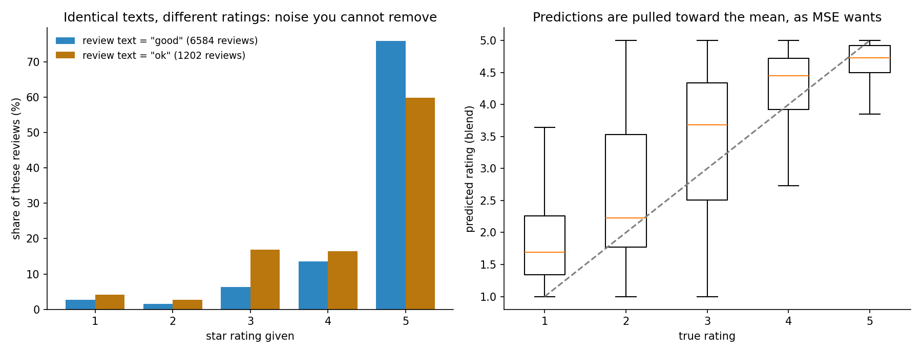
The labels are noisy. The exact same text gets very different ratings: among the 6584 reviews that just say "good", 76 % gave 5 stars but 14 % gave 4 and 6 % gave 3. Over all texts that occur at least 5 times, the spread of ratings within the same text corresponds to an MSE of about 0.6. No model can beat that on those reviews, which tells us that the "best" reference of 0.5 is extremely ambitious.

Left: for reviews whose whole text is "good" or "ok", the share of each star rating; most "good" reviews are 5 stars but every rating occurs. Right: box plots of our blended predictions for each true rating; predictions increase with the true rating but are pulled toward 4 to 5, especially for the rare 2 and 3 stars.

A first baseline

A bag-of-words model is the natural start: TF-IDF features of word unigrams and bigrams plus character 2- to 5-grams (robust to typos such as "Perfct" and "varify"), and a ridge regression on top. This gives an MSE of 0.984 (83.9 points), a huge step from the constant (35). It is quick, and it already captures most of the sentiment words.

Is a hand-built model allowed? The statement restricts pretrained models to BERT; TF-IDF + ridge is trained from scratch on the given data, so we consider it allowed, but we also report the BERT-only result in case it is not.

The key idea

Fine-tune the pretrained model end to end instead of using it as a frozen feature extractor. We first tried the cheap way: compute BERT's sentence vectors once (CLS token and mean of the last layer, 1536 numbers) and fit a ridge regression or a small MLP on them. It was worse than TF-IDF (1.071 and 1.006). BERT was pretrained to predict masked words, not ratings; its frozen vectors mix sentiment with topic, length and syntax, and a linear model on top cannot pull them apart well.

Fine-tuning changes every weight of BERT a little in the direction that reduces our MSE. We add one linear layer on the mean-pooled last hidden states,

\hat y = \mathbf{w}^\top \Big(\frac{1}{T}\sum_{t=1}^{T} \mathbf{h}_t\Big) + b + 3.9,

(the constant 3.9 starts the predictions at the mean rating so early gradients are not wasted) and train everything with the MSE loss, AdamW at a small learning rate ( $3\times10^{-5}$ , one-cycle schedule, gradient clipping) for a single epoch. A small learning rate matters: large updates would destroy the language knowledge we want to reuse. Because of our compute budget we fine-tuned on only 40 000 reviews with at most 64 tokens (roughly 250 characters; 97 % of the reviews are shorter than 300 characters); it still reached 0.896.

Then blend two different models. The fine-tuned BERT and the TF-IDF model make partly independent mistakes (one reads meaning, the other exact character patterns), so their average is better than either:

\hat y = \text{clip}_{[1,5]}\big(0.7\,\hat y_{\text{BERT}} + 0.3\,\hat y_{\text{TF-IDF}}\big).

Clipping to $[1, 5]$ can only help, since the true rating is always in that range. To check that choosing the weight 0.7 on the validation set does not flatter us, we picked it on one half of the validation set and evaluated it on the other half: 0.871, close to the 0.863 on the full validation set.

Why do the predictions look "timid" in the figure (a 2-star review is often predicted around 2.2 to 3.5)? Under MSE, the best prediction is the conditional mean of the rating given the text. When a text is ambiguous, hedging toward the frequent 4 and 5 stars is the right decision, not a bug.

The full solution

Hold out 40 000 random reviews for validation.
TF-IDF (word 1-2-grams, 400k features; character 2-5-grams, 400k features, sublinear term frequency) and ridge ( $\alpha = 3$ ).
Fine-tune bert-base-uncased with a mean-pooling regression head on 40 000 training reviews: batch 32, 1250 steps, about 10 minutes on an Apple GPU.
Predict the validation and test sets (length-sorted batches to minimise padding), blend 0.7/0.3, clip, print.

h = self.bert(**enc).last_hidden_state                  # (batch, tokens, 768)
m = enc["attention_mask"].unsqueeze(-1).float()
pred = self.head((h * m).sum(1) / m.sum(1)).squeeze(1) + 3.9
loss = ((pred - target) ** 2).mean()                     # train the metric itself

Results

Validation MSE on 40 000 held-out reviews (official test labels are private):

approach	validation MSE	score
predict 3 everywhere	3.247	8.4
predict the mean rating	2.439	35.4
TF-IDF words + characters, ridge	0.984	83.9
frozen BERT vectors + ridge (failed idea)	1.071	81.0
frozen BERT vectors + MLP	1.006	83.1
fine-tuned BERT (40k reviews, 1 epoch)	0.896	86.8
blend 0.7 BERT + 0.3 TF-IDF (final)	0.863	87.9
same, weight chosen on the other half of validation	0.871	87.6

The remaining gap to the "best" reference (0.5) is mostly label noise: identical texts alone disagree with an MSE of about 0.6. Fine-tuning on all 200 000 training reviews and for 2 to 3 epochs is the obvious next step (and would probably bring the BERT model alone below 0.85); we stopped at 40 000 reviews to respect the shared compute budget.

What to remember

Measure the noise floor. When identical inputs have different labels, the within-group variance is a lower bound on the MSE; it tells you when to stop.
Fine-tune, do not just freeze. Frozen BERT features were worse than TF-IDF here; end-to-end fine-tuning with a small learning rate was the biggest single gain.
Train on the metric: with MSE scoring, use an MSE loss and a regression head; the optimal prediction is the conditional mean, so hedged predictions are expected.
Blend diverse models and clip to the valid range: a classical TF-IDF model still adds value next to a transformer.
Validate your validation: choose blend weights on one half, check on the other, to make sure the tuning did not leak into the reported number.

"""SAIO "Michaelin Suns": predict a review's star rating (MSE).

Pipeline (validation = 40 000 random training reviews held out):
  A. TF-IDF (word 1-2-grams + character 2-5-grams) + ridge regression.
  B. bert-base-uncased (the one pretrained model allowed) fine-tuned end to end
     as a regressor: mean-pooled last layer -> linear head, MSE loss, AdamW 3e-5,
     one epoch on 40 000 reviews (max 64 tokens), Apple MPS.
  C. blend 0.7 * B + 0.3 * A, clipped to [1, 5].
Kattis receives the predictions printed by the submitted program.

Run: python solution.py data/       (writes val/test predictions and answer.txt)
"""
import sys, time
import numpy as np
import pandas as pd
import torch
from scipy.sparse import hstack
from sklearn.feature_extraction.text import TfidfVectorizer
from sklearn.linear_model import Ridge
from transformers import BertModel, BertTokenizer

torch.set_num_threads(2); torch.manual_seed(0)
DATA = sys.argv[1] if len(sys.argv) > 1 else "data/"
DEV = "mps" if torch.backends.mps.is_available() else "cpu"
N_FT, MAXLEN, BATCH, LR, W_BERT = 40000, 64, 32, 3e-5, 0.7

d = pd.read_csv(DATA + "train.csv"); t = pd.read_csv(DATA + "test.csv")
txt = d.content.fillna("").astype(str).values; ttxt = t.content.fillna("").astype(str).values
y = d.rating.values.astype(np.float32)
rng = np.random.default_rng(0)
perm = rng.permutation(len(d)); va, tr = perm[:40000], perm[40000:]
mse = lambda p, yy: float(((np.clip(p, 1, 5) - yy) ** 2).mean())
score = lambda m: max(0.0, min(100.0, (3.5 - m) / 3.0 * 100))

# ---------------------------------------------------------------- A. TF-IDF + ridge
w = TfidfVectorizer(ngram_range=(1, 2), min_df=2, max_features=400000, sublinear_tf=True)
c = TfidfVectorizer(analyzer="char_wb", ngram_range=(2, 5), min_df=3, max_features=400000, sublinear_tf=True)
X = hstack([w.fit_transform(txt[tr]), c.fit_transform(txt[tr])]).tocsr()
feat = lambda s: hstack([w.transform(s), c.transform(s)]).tocsr()
ridge = Ridge(alpha=3).fit(X, y[tr])
va_a, te_a = ridge.predict(feat(txt[va])), ridge.predict(feat(ttxt))
print(f"constant mean: {mse(np.full(len(va), y[tr].mean()), y[va]):.3f}")
print(f"A tfidf+ridge: {mse(va_a, y[va]):.3f}")

# ---------------------------------------------------------------- B. fine-tuned BERT
tok = BertTokenizer.from_pretrained("bert-base-uncased")


class Regressor(torch.nn.Module):
    def __init__(self):
        super().__init__()
        self.bert = BertModel.from_pretrained("bert-base-uncased")
        self.head = torch.nn.Linear(768, 1)

    def forward(self, **enc):
        h = self.bert(**enc).last_hidden_state
        m = enc["attention_mask"].unsqueeze(-1).float()
        return self.head((h * m).sum(1) / m.sum(1)).squeeze(1) + 3.9   # start near the mean


net = Regressor().to(DEV)
sub = rng.permutation(tr)[:N_FT]
steps = len(sub) // BATCH
opt = torch.optim.AdamW(net.parameters(), lr=LR, weight_decay=0.01)
sched = torch.optim.lr_scheduler.OneCycleLR(opt, LR, total_steps=steps, pct_start=0.06)
net.train(); t0 = time.time()
for s in range(steps):
    b = sub[s * BATCH:(s + 1) * BATCH]
    enc = tok(list(txt[b]), padding=True, truncation=True, max_length=MAXLEN, return_tensors="pt").to(DEV)
    loss = ((net(**enc) - torch.tensor(y[b], device=DEV)) ** 2).mean()
    opt.zero_grad(); loss.backward()
    torch.nn.utils.clip_grad_norm_(net.parameters(), 1.0); opt.step(); sched.step()
    if s % 200 == 0:
        print(f"step {s}/{steps} loss {loss.item():.3f} {time.time() - t0:.0f}s", flush=True)


@torch.no_grad()
def predict(texts):
    net.eval(); order = np.argsort([len(x) for x in texts]); out = np.zeros(len(texts), np.float32)
    for i in range(0, len(texts), 256):          # length-sorted batches: little padding
        idx = order[i:i + 256]
        enc = tok([texts[j] for j in idx], padding=True, truncation=True, max_length=128,
                  return_tensors="pt").to(DEV)
        out[idx] = net(**enc).float().cpu().numpy()
    return out


va_b, te_b = predict(list(txt[va])), predict(list(ttxt))
print(f"B fine-tuned BERT: {mse(va_b, y[va]):.3f}")

# ---------------------------------------------------------------- C. blend
va_c = W_BERT * va_b + (1 - W_BERT) * va_a
m = mse(va_c, y[va]); print(f"C blend: {m:.3f}  -> score {score(m):.1f}")
pred = np.clip(W_BERT * te_b + (1 - W_BERT) * te_a, 1, 5)
open("answer.txt", "w").write("\n".join(f"{p:.3f}" for p in pred) + "\n")