Sweden SAIO · Correction by IOAI Training

Disaster in Chongmetry

This page gives the full approach. Read it once you have searched.

Metric: capped mean absolute error D
Evaluated on: held-out validation (official test labels are private)
Our score: D = 0.129 (about 93/100 points)
Expected level: 100 points at D <= 0.1; 0 points at D = 0.5

Our solution does not reach the expected level: there is still room to beat it

We solved the problem ourselves: downloaded the data, ran the experiments and measured the score below. The statement and data belong to their organisers.

The problem in brief

Each of 200 bridges is a curve $y = f(x)$ on $0 \le x \le 10$ . For every bridge you are given about 70 surviving points $(x, y)$ , and the $x$ positions (15 to 47 of them) where pillars must be rebuilt. These positions all fall inside one contiguous broken stretch, typically 2 to 4 metres wide, with no surviving point inside it. You must output the missing heights. The statement hints at the twist: the city is "built from mathematical formulas".

How you are scored

With $n$ test positions, the error of each prediction is capped at 0.5 and averaged:

D = \frac{1}{n}\sum_{i=1}^{n} \min\big(0.5,\ |y_i - \hat y_i|\big), \qquad \text{Score} = \max\Big(0, \min\Big(100,\ 100\cdot\frac{0.5 - D}{0.5 - 0.1}\Big)\Big).

So $D = 0.5$ (completely wrong everywhere) gives 0 points and $D \le 0.1$ gives the full 100 points: that is the target. The cap means a hopeless bridge costs at most 0.5, so it pays to be exactly right on as many bridges as possible rather than roughly right everywhere. The true heights are hidden on Kattis; we estimate $D$ ourselves (see Results).

First look at the data

Plotting a few bridges is the most important step of this problem.

The shapes are textbook functions: parabolas, cubics, clean sinusoids, decaying oscillations, S-curves, bumps, kinks, staircases.
For every bridge the $y$ values have mean exactly 0 and standard deviation exactly 1 over the training points: the organisers standardised $y$ . That is only an affine change $y = (f(x) - \mu)/\sigma$ , so any family with a free scale and offset absorbs it.
The decisive test: fit a degree-2 polynomial to bridge 0 and the residual is $10^{-16}$ , machine precision. There is no noise at all. The surviving points are exact samples of a closed-form formula.

That observation changes the nature of the problem. The provided example solution copies the height of the nearest surviving point, and generic interpolation (splines) just draws a smooth bridge across the hole. Both are guessing. If we can recognise the formula, we can compute the hole exactly.

A first baseline

To measure anything without the hidden answers we need our own test. For each bridge we hide the known points lying just next to the real broken stretch (a fake gap of the same width) and predict them from the remaining points. This is harder than the real task, since the fake gap is glued to the real one (the hole to bridge is twice as wide), so our estimates are pessimistic.

baseline	estimated $D$	estimated score
nearest surviving point (the organisers' example notebook)	0.375	31
shape-preserving cubic interpolation (PCHIP)	0.321	45

Interpolation fails exactly where it matters: a sine wave has a whole trough inside the gap, and a spline cannot know it is there.

The key idea

No noise means a correct model fits perfectly, and a wrong model does not. With 70 exact points, a family with 3 to 7 parameters either reproduces them to $10^{-10}$ or misses them by $10^{-3}$ or more. There is almost nothing in between: the figure below shows the training RMSE of the best family for each bridge, and it splits into two clean worlds separated by a valley around $10^{-6}$ .

Histogram of log10 of the training RMSE of the best family for each of the 200 bridges. One group sits between 1e-16 and 1e-7 (formula identified), another between 1e-5 and 1 (not in the library), with an empty gap around the threshold 1e-6.

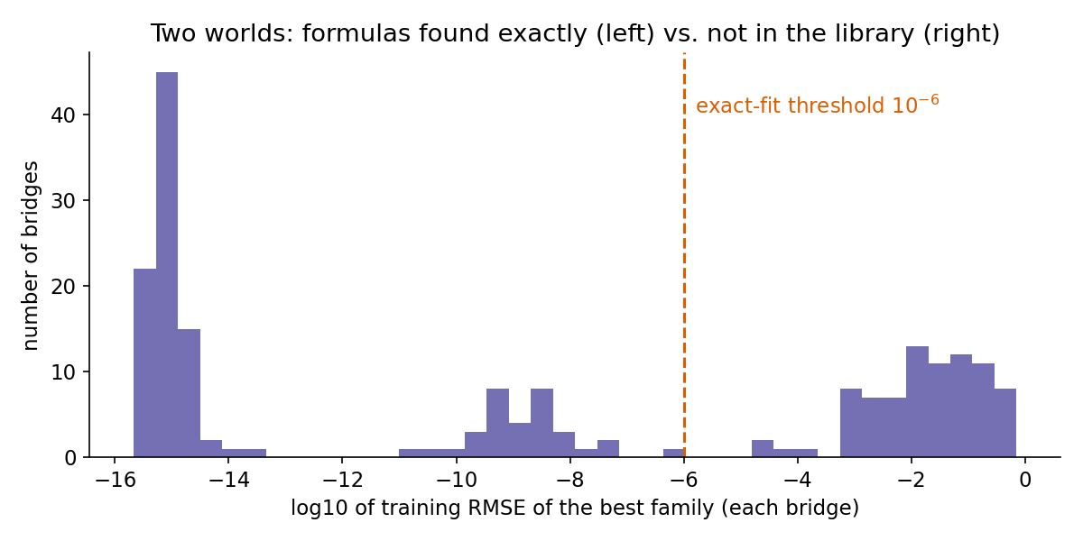
So the method is model identification rather than regression:

Build a library of families: polynomials of degree 1 to 8, $a\sin(\omega x+\varphi)+d$ , the same plus a linear trend, damped oscillations $a e^{kx}\sin(\omega x+\varphi)+d$ , chirps $a\sin(ux^2+\omega x+\varphi)+d$ , sums of two sines, amplitude-modulated sines, $a\tanh(b(x-c))+d$ , Gaussian and Laplace bumps, exponentials, kinks $a|x-c|+bx+d$ and squared ReLUs.
Fit each family to the surviving points by least squares.
If some families fit to RMSE $< 10^{-6}$ , take the one with fewest parameters (Occam's razor: a parabola also "is" a degree-8 polynomial, but the simplest exact explanation is the one to trust).
Otherwise (no family is exact), choose between the families that fit decently, PCHIP interpolation and nearest neighbour by how well each refills pseudo-gaps cut out next to the real gap.

Why is an exact fit trustworthy? If a family with $k$ parameters passes through $70 \gg k$ exact points, the chance that a different function does so by coincidence is negligible: each extra point is an extra equation the coincidence would have to satisfy. Fitting is cheap, and the test is binary.

The one technical difficulty is that the non-linear fits have local minima. A sine fit started at the wrong frequency converges to a wrong, smaller wiggle. Two cures are used:

For oscillating families, scan a grid of 1 200 frequencies $\omega$ ; for a fixed $\omega$ the model $A\sin\omega x + B\cos\omega x + d$ is linear in $(A, B, d)$ , so each grid point is a tiny least-squares solve. The best $\omega$ seeds curve_fit, which refines all parameters together.
For S-curves, bumps and kinks, start curve_fit from a deterministic grid of centres $c$ , widths and signs, and keep the best.

fits = {name: fit_family(name, x, y) for name in FAMILIES}      # (train RMSE, predictor)
exact = [n for n, (rmse, g) in fits.items() if rmse < 1e-6]
if exact:
    best = min(exact, key=lambda n: N_PARAMS[n])                 # Occam
    return fits[best].predict(x_gap)

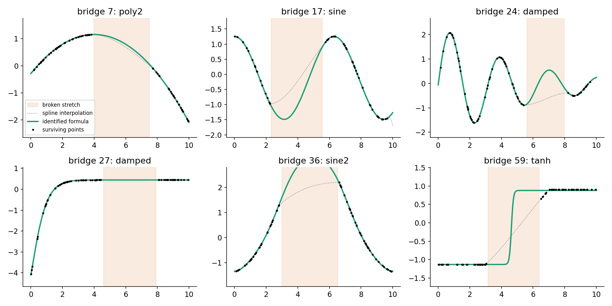
Look at bridges 17 and 24: the spline draws a gentle slope across the gap while the true curve dips through a full trough or crest. Those are exactly the points where the capped error would have been 0.5.

The full solution

solution.py (about 150 lines, NumPy and SciPy only):

For each bridge, sort the surviving points and compute the gap width from the test positions.
Fit the 22 families (8 polynomials and 14 non-linear forms) with the start strategies above.
Exact fit found: predict with the simplest exact family (119 of the 200 bridges).
No exact fit: for each candidate that fits all points with RMSE below 0.05, plus PCHIP and nearest neighbour, hide a window of the gap's width just left and just right of the real gap, refit, and measure the capped error; keep the candidate with the smallest average.
Print one height per line, in the order of test.csv.

The whole run takes about 3 minutes on one CPU core.

Results

Estimated on the pseudo-gap protocol described above (the real answers are private; Kattis also re-scores on a hidden 70 % at the end of the contest):

approach	estimated $D$	estimated score
nearest surviving point (example solution)	0.375	31
PCHIP interpolation	0.321	45
one global polynomial per bridge, degree 3 / 6 / 8	0.273 / 0.223 / 0.204	57 / 69 / 74
formula identification + pseudo-gap fallback	0.129	93

Where the remaining error lives: the identified formulas are exact on 129 of the 200 validation gaps, covering 63 % of the hidden points, with error $10^{-8}$ or less. On the other 71 bridges (staircases, square waves, aliased high-frequency curves, shapes outside the library) the fallback reaches $D = 0.35$ , barely better than PCHIP (0.37). The score is therefore decided almost entirely by how many formulas you recognise: each extra family that matches a group of bridges converts a 0.35 error into 0. Further gains would come from adding the missing families (floors and sign functions for the staircases, compositions such as $\sin(e^{x})$ for the very irregular ones).

A detail that cost us a bug: with random restarts, the same bridge was sometimes identified and sometimes not. Deterministic start grids made the method reproducible, which matters when a contest re-runs your code.

What to remember

Plot first, and test for noise. A residual of $10^{-16}$ tells you that you are not doing statistics but recovering an exact law; the right tool changes completely.
Exact data turns model selection into a yes/no test: a family that reproduces many exact points with few parameters is the formula. Prefer the simplest exact explanation.
Non-linear least squares needs good starts. Scan the hard parameter (here the frequency) on a grid, solve the linear part exactly at each grid point, then refine.
Build your own validation that mimics the test. Here: hide a contiguous stretch of known points next to the real gap, never random isolated points, which would make interpolation look far too good.
Know your metric. A capped error rewards being exactly right on many items more than being approximately right on all.

Full code (solution.py)

"""SAIO "Disaster in Chongmetry": fill the missing stretch of each bridge curve.

Key observation: the surviving points are EXACT samples of a closed-form function (no noise; y is only
standardised). So instead of interpolating, we identify the formula:
  1. fit a library of parametric families (polynomials, sines, chirps, sigmoids, bumps, kinks, ...)
     to the surviving points, from a deterministic grid of starting points (non-linear fits have
     local minima: one start is not enough);
  2. a family that reproduces the points to ~1e-6 is (almost surely) the true formula: keep the
     simplest such family (fewest parameters), Occam's razor;
  3. if no family is exact, choose the one that best predicts artificially removed stretches
     (a pseudo-gap of the same width as the real one), with shape-preserving interpolation in the pool.

  python solution.py --val    honest estimate: hide a stretch of known points next to the real gap
  python solution.py          write the predictions for test.csv (one y per line) to work/out.txt
"""
import sys, warnings
import numpy as np, pandas as pd
from scipy.optimize import curve_fit
from scipy.interpolate import PchipInterpolator
warnings.filterwarnings("ignore")

def cap_err(p, y): return float(np.minimum(0.5, np.abs(p - y)).mean())

# ----------------------------------------------------------------- the library of families
# each entry: name -> (model(x, *p), number of params, initial-guess generator(x, y))
def _amp(y): return (y.max() - y.min()) / 2
CS = np.linspace(0.5, 9.5, 10)                       # grid of start positions for kinks / centres
FAMILIES = {
    "tanh":     (lambda x, a, b, c, d: a * np.tanh(b * (x - c)) + d, 4,
                 lambda x, y: [[sg * _amp(y), b, c, y.mean()] for sg in (-1, 1) for b in (0.5, 2, 6) for c in CS]),
    "gauss":    (lambda x, a, c, s, d: a * np.exp(-((x - c) / s) ** 2) + d, 4,
                 lambda x, y: [[sg * 2 * _amp(y), c, s, y.mean()] for sg in (-1, 1) for s in (0.7, 2, 5) for c in CS]),
    "laplace":  (lambda x, a, c, s, d: a * np.exp(-np.abs(x - c) / s) + d, 4,
                 lambda x, y: [[sg * 2 * _amp(y), c, s, y.mean()] for sg in (-1, 1) for s in (0.7, 2, 5) for c in CS]),
    "exp":      (lambda x, a, b, d: a * np.exp(b * x) + d, 3,
                 lambda x, y: [[sg, b, y.mean()] for sg in (-1, 1) for b in (-2, -0.7, -0.2, 0.2, 0.7, 2)]),
    "kink":     (lambda x, a, b, c, d: a * np.abs(x - c) + b * x + d, 4,
                 lambda x, y: [[1, 0, c, y.mean()] for c in CS]),
    "relu2":    (lambda x, a, c, b, d: a * np.maximum(0, x - c) ** 2 + b * x + d, 4,
                 lambda x, y: [[sg, c, 0, y.mean()] for sg in (-1, 1) for c in CS]),
    "sine":     (lambda x, a, w, p, d: a * np.sin(w * x + p) + d, 4, None),           # frequency grid
    "sine_lin": (lambda x, a, w, p, b, d: a * np.sin(w * x + p) + b * x + d, 5, None),
    "damped":   (lambda x, a, k, w, p, d: a * np.exp(k * x) * np.sin(w * x + p) + d, 5, None),
    "chirp":    (lambda x, a, u, w, p, d: a * np.sin(u * x ** 2 + w * x + p) + d, 5, None),
    "sine2":    (lambda x, a, w, p, b, v, q, d: a * np.sin(w * x + p) + b * np.sin(v * x + q) + d, 7, None),
    "sine_x":   (lambda x, a, w, p, b, d: (a + b * x) * np.sin(w * x + p) + d, 5, None),
}
for deg in range(1, 9):
    FAMILIES[f"poly{deg}"] = (None, deg + 1, None)

def best_sine_start(x, y, wmax=40):
    """Linear least squares on a frequency grid: y ~ A sin(wx) + B cos(wx) + d. Returns (w, a, p, d)."""
    best = (np.inf, None)
    for w in np.linspace(0.1, wmax, 1200):
        A = np.stack([np.sin(w * x), np.cos(w * x), np.ones_like(x)], 1)
        c, *_ = np.linalg.lstsq(A, y, rcond=None); r = ((A @ c - y) ** 2).sum()
        if r < best[0]: best = (r, (w, np.hypot(c[0], c[1]), np.arctan2(c[1], c[0]), c[2]))
    return best[1]

def starts(name, x, y):
    if FAMILIES[name][2] is not None:
        return FAMILIES[name][2](x, y)
    w, a, p, d = best_sine_start(x, y)
    if name == "sine":     return [[a, w, p, d]]
    if name == "sine_lin": return [[a, w, p, 0.0, d]]
    if name == "damped":   return [[a, k_, w, p, d] for k_ in (-0.3, 0.0, 0.3)]
    if name == "sine_x":   return [[a, w, p, 0.0, d]]
    if name == "chirp":    return [[a, u, w - 10 * u, p, d] for u in (-0.3, -0.1, 0.05, 0.1, 0.3, 1.0)]
    if name == "sine2":    # second component fitted on the residual of the first
        r = y - a * np.sin(w * x + p) - d; w2, b, q, _ = best_sine_start(x, r)
        return [[a, w, p, b, w2, q, d]]

def fit_family(name, x, y):
    """Return (train RMSE, predictor) of the best restart."""
    if name.startswith("poly"):
        deg = int(name[4:]); c = np.polyfit(x, y, deg)
        return np.sqrt(((np.polyval(c, x) - y) ** 2).mean()), lambda q: np.polyval(c, q)
    f = FAMILIES[name][0]; best = (np.inf, None)
    for p0 in starts(name, x, y):
        try:
            p, _ = curve_fit(f, x, y, p0=p0, maxfev=4000)
            r = np.sqrt(((f(x, *p) - y) ** 2).mean())
            if np.isfinite(r) and r < best[0]: best = (r, p)
        except Exception:
            pass
    if best[1] is None: return np.inf, None
    p = best[1]; return best[0], (lambda q: f(q, *p))

def interp_pchip(x, y):
    return PchipInterpolator(x, y, extrapolate=True)

EXACT = 1e-6

def predict(x, y, q, gap_w, depth=1, gap=None):
    """Full decision procedure for one bridge: points (x, y) -> heights at q (gap = (lo, hi) of the hole)."""
    fits = {n: fit_family(n, x, y) for n in FAMILIES}
    exact = [n for n, (r, _) in fits.items() if r < EXACT and fits[n][1] is not None]
    if exact:                                             # Occam: fewest parameters among exact fits
        n = min(exact, key=lambda n: FAMILIES[n][1])
        return fits[n][1](q), n
    if depth == 0:                                        # inside the pseudo-gap selection itself
        return None, None
    # no exact formula: pick the candidate that best refills pseudo-gaps cut out of the known points
    lo, hi = gap if gap is not None else (q.min(), q.max())
    # a family is only a candidate if its fit on ALL points is decent (a lucky fit on the reduced
    # points of a pseudo-gap is useless if the final fit lands in a bad local minimum)
    cands = [n for n, (r, g) in fits.items() if g is not None and r < 0.05] + ["pchip", "nearest"]
    scores = {c: [] for c in cands}
    for side in (-1, 1):
        c0 = lo - gap_w / 2 - 0.05 if side < 0 else hi + gap_w / 2 + 0.05
        m = (x > c0 - gap_w / 2) & (x < c0 + gap_w / 2)
        if m.sum() < 3 or (~m).sum() < 10: continue
        xa, ya = x[~m], y[~m]
        for c in cands:
            if c == "pchip": p = interp_pchip(xa, ya)(x[m])
            elif c == "nearest": p = ya[np.abs(x[m][:, None] - xa[None]).argmin(1)]
            else:
                r, g = fit_family(c, xa, ya); p = g(x[m]) if g is not None else np.full(m.sum(), ya.mean())
            scores[c].append(cap_err(p, y[m]))
    scored = {c: np.mean(v) for c, v in scores.items() if v}
    if not scored: return interp_pchip(x, y)(q), "pchip"
    c = min(scored, key=scored.get)
    if c == "pchip" or fits.get(c, (0, None))[1] is None: return interp_pchip(x, y)(q), "pchip"
    if c == "nearest": return y[np.abs(q[:, None] - x[None]).argmin(1)], c
    return fits[c][1](q), c

if __name__ == "__main__":
    tr = pd.read_csv("work/data/train.csv"); te = pd.read_csv("work/data/test.csv")
    val = "--val" in sys.argv
    out, rows = [], []
    for f in sorted(tr.function_id.unique()):
        d = tr[tr.function_id == f].sort_values("x"); x, y = d.x.values, d.y.values
        q = te[te.function_id == f].x.values; gw = q.max() - q.min()
        if val:
            # hide the known points just right (or left) of the real gap, same width: a fake gap
            lo, hi = q.min(), q.max()
            right = (x > hi) & (x < hi + gw); left = (x < lo) & (x > lo - gw)
            m = right if right.sum() >= left.sum() else left
            p, how = predict(x[~m], y[~m], x[m], gw)
            nn = y[~m][np.abs(x[m][:, None] - x[~m][None]).argmin(1)]
            rows.append({"f": f, "how": how, "D": cap_err(p, y[m]), "D_nearest": cap_err(nn, y[m]),
                         "D_pchip": cap_err(interp_pchip(x[~m], y[~m])(x[m]), y[m]), "n": int(m.sum())})
            print(rows[-1], flush=True)
        else:
            p, how = predict(x, y, q, gw); out.extend(p.tolist()); print(f, how, flush=True)
    if val:
        r = pd.DataFrame(rows); r.to_csv("work/val.csv", index=False)
        w = r.n / r.n.sum()
        for c in ["D", "D_nearest", "D_pchip"]:
            D = (r[c] * w).sum(); print(c, round(D, 4), "score", round(max(0, min(100, (0.5 - D) / 0.4 * 100)), 1))
        print(r.how.value_counts())
    else:
        open("work/out.txt", "w").write("\n".join(f"{v:.10f}" for v in out) + "\n")