IOAI Training: Learn AI by solving problems

The problem in brief

Screenshots were taken at random places in a $2500 \times 2500$ Minecraft world. For 774 of them you know the position $(x, z)$ where they were taken, plus the camera's yaw (left-right rotation) and pitch (up-down). For 952 others you only have the image, the yaw and the pitch, and you must say where the camera was. The images are tiny ( $128\times74$ or $64\times37$ pixels) and no two screenshots share a position. It is a visual geolocation problem, like guessing the country from a street photo.

How you are scored

With $\bar d$ the mean Euclidean distance between predicted and true positions,

\text{Points} = \min\!\Big(100,\ \max\!\Big(0,\ 100\cdot\frac{1000 - \bar d}{1000 - 400}\Big)\Big).

So $\bar d = 1000$ gives 0 points and $\bar d \le 400$ gives 100 points. The Kattis program must run in 1 second, so in practice you compute the predictions offline and submit a program that prints them. The true positions of the test images are hidden; we estimate $\bar d$ with 5-fold cross-validation on the 774 labelled screenshots.

First look at the data

The training positions cover the map uniformly, with a typical spacing of about 40 blocks between neighbouring screenshots: no two images show exactly the same spot.
Always answering the centre of the map gives $\bar d = 953$ , 8 points. That is the score of knowing nothing.
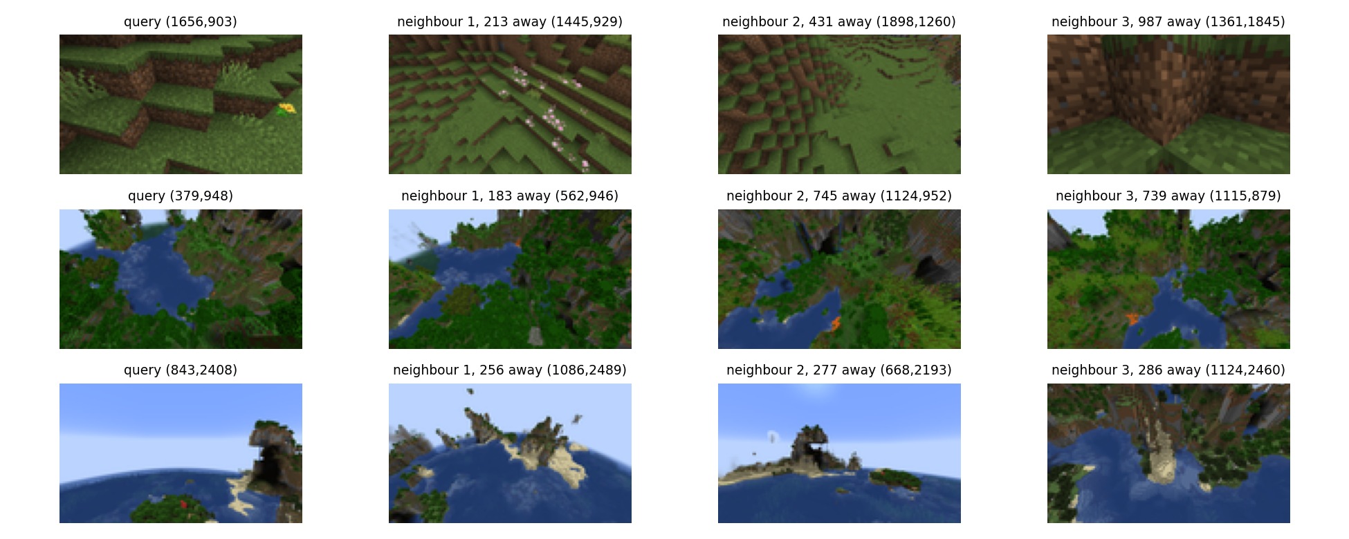
Looking at the images, what changes with position is not objects but the landscape palette: green plains, dark jungle, blue ocean with sandy islands, snowy mountains, orange mesa. Minecraft generates biomes, large regions of a few hundred blocks with a characteristic look.
Many screenshots are mostly sky (high pitch or a view over the sea), and the sky is the same blue everywhere.

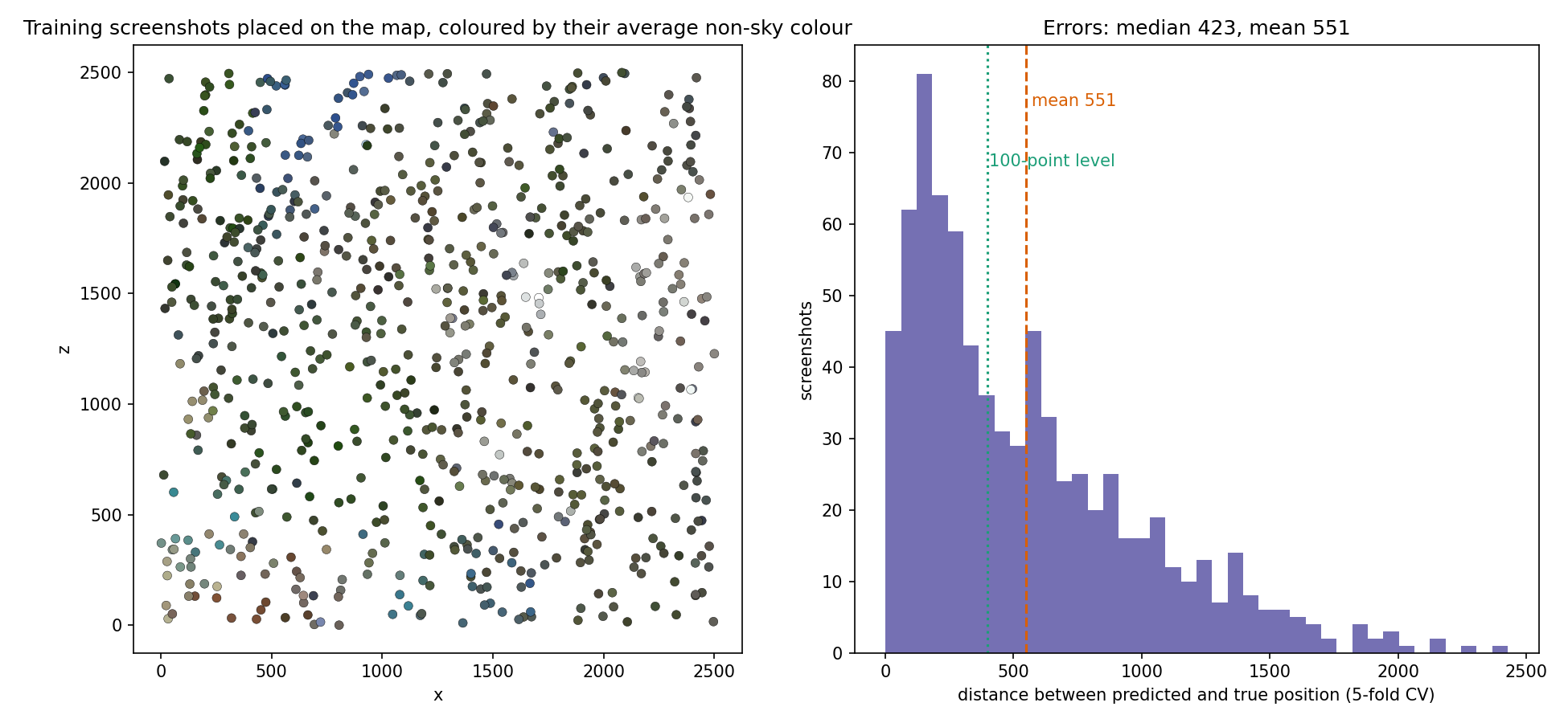
Left: the 774 training screenshots placed at their true position, each dot coloured by the average colour of its non-sky pixels: neighbouring dots tend to share colours (blue patches near the top and bottom-left, grey in the centre-right, green elsewhere). Right: histogram of the cross-validated prediction errors of the final model, median 423, mean 551.

The left map is the whole idea: colour is a (weak) function of position. Nearby screenshots look alike because they are in the same biome.

A first baseline

The natural first try for "find similar images" is a pretrained CNN. We describe each screenshot by the 512-dimensional pooled features of an ImageNet ResNet-34 and predict the position of the most similar training image (cosine similarity, 1-nearest neighbour).

approach (5-fold CV)	$\bar d$	points
always the map centre	953	8
ResNet-34 features, 1 nearest neighbour	973	5
ResNet-34 features, weighted average of 10 neighbours	788	35

The 1-NN is worse than guessing the centre. Two lessons. First, ImageNet features describe objects and shapes (a "mountain", a "tree"), which exist everywhere in the world; they barely encode which green or which sand. Second, under a mean-distance metric, committing to one neighbour is risky: a wrong match costs up to 2 500, while averaging several plausible neighbours hedges toward the middle of the candidate area.

The key idea

Describe the image by its colour distribution, without the sky, and average the positions of the most similar screenshots.

Convert to HSV and quantise each channel into 16 levels, giving $16^3 = 4096$ colour bins. Fine bins matter: Minecraft blocks have exact, repeated colours, so "this exact green of jungle leaves" is a strong clue that coarse bins blur away.
Drop the sky pixels (bright, blue hue, moderate saturation) before counting: they carry no information about position and, depending on the pitch, can fill most of the image, which would make every high-pitch screenshot look like every other.
Compare histograms with the Hellinger similarity: take the square root of each normalised histogram, L2-normalise, and use the dot product. The square root damps dominant colours so that a small patch of sand or snow still counts.
Predict with a soft $k$ -nearest-neighbour regression: take the $k = 10$ most similar training screenshots and average their positions with weights $w_j \propto \exp\big((s_j - s_{\max})/\tau\big)$ , $\tau = 0.02$ , where $s_j$ is the similarity.

Why averaging is right for this metric: if the evidence says "this is jungle, and jungle exists in three regions", the point that minimises the expected distance lies between those regions (it is the geometric median of the plausible positions; the weighted mean is a simple stand-in for it), not in one of them. Small $\tau$ trusts close matches; larger $k$ and $\tau$ hedge more. We also tried pulling predictions further toward the map centre, and it only hurt (from 551 to 560 with 10 % shrinkage): the neighbour averaging already hedges enough.

Three query screenshots and their three most similar training screenshots by colour histogram, with the distance between their true positions. A grassy hill matches other grass at 213 and 431 blocks; a jungle lake matches a jungle lake 183 blocks away, then two from 740 blocks away; an ocean view with sandy islands matches three ocean views 256 to 286 blocks away.

The full solution

solution.py (about 80 lines):

q = np.minimum(hsv.reshape(-1, 3) * 16 // 256, 15)          # 16 levels per channel
q = q[~is_sky(hsv).reshape(-1)]                              # drop sky pixels
h = np.bincount(q[:, 0] * 256 + q[:, 1] * 16 + q[:, 2], minlength=4096)
f = np.sqrt(h / h.sum()); f /= np.linalg.norm(f)             # Hellinger embedding
S = F_test @ F_train.T                                       # cosine similarities
# 10 best neighbours, softmax weights with temperature 0.02, weighted mean of their (x, z)

The predictions are computed once (seconds on a CPU) and written as $x$ then $z$ for each test image, which a trivial program prints within Kattis's 1-second limit. Yaw and pitch are not used by the final model; we only exploit pitch indirectly, by removing the sky that high-pitch views are full of.

Results

5-fold cross-validation on the 774 labelled screenshots (the official test positions are private):

approach	$\bar d$	estimated points
map centre	953	8
ResNet-34 features, 1-NN	973	5
ResNet-34 features, $k=10$	788	35
HSV histogram, 6 levels per channel, $k=10$	662	56
HSV histogram, 16 levels, $k=10$	601	67
16 levels, sky removed, $k=10$ , $\tau=0.02$ (final)	551	75
same + 10 % of ResNet features in the similarity	550	75
same + shrink 10 % toward the centre	560	73

The errors are very unequal (right panel of the first figure): the median is 423, almost the 100-point level, and 48 % of the screenshots are placed within 400 blocks, but a tail of confusions between distant regions of the same biome costs more than 1 000 each and pulls the mean up to 551. Reaching 400 on average would need cues that tell apart two forests of the same type: the shapes of specific landmarks, or a model that uses yaw and pitch to know which direction it is looking (a learned image embedding trained on these 774 images, with augmentations, is the natural next step).

What to remember

Ask what actually varies with the target. Here it is the colour palette of biomes, not objects, so a hand-crafted colour histogram beats ImageNet features by a wide margin.
Remove the parts of the input that carry no signal (the sky): it makes similarities meaningful.
Fine quantisation and a square-root (Hellinger) transform are cheap ways to make histograms discriminative and robust.
Match the prediction rule to the metric. For a mean distance, a weighted average of several plausible neighbours beats the single nearest neighbour.
Validate the way you are tested: cross-validated mean distance, converted to points with the official formula, before ever submitting.

"""SAIO final 2025 "Chicken Jockey": where in a 2500 x 2500 Minecraft world was this screenshot taken?

Pipeline: describe each 128x74 screenshot by
  * a fine HSV colour histogram of the NON-sky pixels (biomes have colours: snow, sand, jungle,
    ocean, mesa), compared with the Hellinger / cosine similarity
  (ImageNet ResNet-34 features were tried and are much worse: they describe objects, not palettes),
then predict (x, z) as a similarity-weighted average of the k most similar training screenshots.
Averaging is deliberate: under a mean-Euclidean-distance metric, when unsure, hedging toward the
centre of the plausible area is better than committing to one wrong neighbour.

  python solution.py --val   5-fold cross-validation on train.csv (test answers are hidden on Kattis)
  python solution.py         write predictions for test.csv to work/out.txt (x then z, one per line)
Data: saio.kattis.com/problems/chickenjockey/file/statement/attachments/data.zip, unzipped in work/.
"""
import sys
import numpy as np, pandas as pd, torch, torchvision
from PIL import Image
from sklearn.model_selection import KFold

torch.set_num_threads(2)
tr = pd.read_csv("work/train.csv", dtype={"id": str}); te = pd.read_csv("work/test.csv", dtype={"id": str})

def load(i): return Image.open(f"work/img_128x74/{int(i)}.png").convert("RGB")

@torch.no_grad()
def cnn_features(ids):
    m = torchvision.models.resnet34(weights=torchvision.models.ResNet34_Weights.DEFAULT); m.fc = torch.nn.Identity(); m.eval()
    tf = torchvision.transforms.Compose([torchvision.transforms.Resize((148, 256)), torchvision.transforms.ToTensor(),
                                         torchvision.transforms.Normalize([0.485, 0.456, 0.406], [0.229, 0.224, 0.225])])
    out = []
    for k in range(0, len(ids), 64):
        out.append(m(torch.stack([tf(load(i)) for i in ids[k:k + 64]])).numpy())
    f = np.concatenate(out); return f / np.linalg.norm(f, axis=1, keepdims=True)

def is_sky(hsv):
    """Sky pixels (blue, bright, not too saturated in PIL's 0-255 HSV) look the same everywhere: drop them."""
    return (hsv[..., 0] > 130) & (hsv[..., 0] < 175) & (hsv[..., 2] > 150) & (hsv[..., 1] < 200)

def colour_features(ids, bins=16, drop_sky=True):
    out = []
    for i in ids:
        hsv = np.asarray(load(i).convert("HSV")).astype(int)
        q = np.minimum(hsv.reshape(-1, 3) * bins // 256, bins - 1)
        if drop_sky: q = q[~is_sky(hsv).reshape(-1)]
        h = np.bincount(q[:, 0] * bins * bins + q[:, 1] * bins + q[:, 2], minlength=bins ** 3).astype(float)
        out.append(np.sqrt(h / max(h.sum(), 1)) + 1e-9)         # Hellinger: sqrt of the histogram
    f = np.array(out); return f / np.linalg.norm(f, axis=1, keepdims=True)

def knn_predict(Ftr, Ytr, Fq, k=10, temp=0.05):
    S = Fq @ Ftr.T                                            # cosine similarity
    idx = np.argsort(-S, 1)[:, :k]; s = np.take_along_axis(S, idx, 1)
    w = np.exp((s - s[:, :1]) / temp)                          # softmax over the k neighbours
    return (w[..., None] * Ytr[idx]).sum(1) / w.sum(1, keepdims=True)

def combine(Fc, Fh, alpha):
    return np.hstack([np.sqrt(1 - alpha) * Fc, np.sqrt(alpha) * Fh])   # cosine of the concatenation = weighted sum

def points(d): return min(100, max(0, 100 * (1000 - d) / 600))

def cv(F, Y, k=10, temp=0.02):
    P = np.zeros_like(Y)
    for a, b in KFold(5, shuffle=True, random_state=0).split(F): P[b] = knn_predict(F[a], Y[a], F[b], k, temp)
    return np.hypot(*(P - Y).T).mean()

if __name__ == "__main__":
    ids_all = list(tr.id) + list(te.id); n = len(tr); Y = tr[["x", "z"]].values.astype(float)
    if "--val" in sys.argv:
        print("predict the mean position:", round(np.hypot(*(Y - Y.mean(0)).T).mean(), 1))
        Fc = cnn_features(list(tr.id))
        rows = [("ResNet-34 features, 1-NN", Fc, 1, 1.0), ("ResNet-34 features, k=10", Fc, 10, 0.05),
                ("HSV histogram 6 bins, k=10", colour_features(tr.id, 6, False), 10, 0.05),
                ("HSV histogram 16 bins, k=10", colour_features(tr.id, 16, False), 10, 0.05),
                ("16 bins, sky removed, k=10", colour_features(tr.id, 16, True), 10, 0.02)]
        for name, F, k, t in rows:
            d = cv(F, Y, k, t); print(f"{name:30s} avg dist {d:6.1f}  points {points(d):5.1f}", flush=True)
    else:
        F = colour_features(ids_all)
        P = knn_predict(F[:n], Y, F[n:], 10, 0.02)
        # Kattis has a 1 s limit: submit a tiny program that just prints these precomputed numbers
        open("work/out.txt", "w").write("".join(f"{int(round(x))}\n{int(round(z))}\n" for x, z in P))