Predicția statusului pacientului

The problem in brief

You receive a table of 3,219 breast-cancer patients (stage of the tumour, lymph nodes, hormone receptors, age, marital status...) plus seventeen vital signs and blood tests, and for each one whether the patient ended up Dead or Alive. A test table of 805 patients comes without the outcome. Four short warm-up subtasks (40 points) ask for exact computations on the test patients: a kidney-function label, a creatinine risk level from quartiles, a BMI flag and a count. The main subtask (60 points) asks you to predict the status, and it is scored only by the precision on the Dead class. The data and statement come from the public mirror of the ROAI 2025 rounds (github.com/jaredliw/ioai-tsp-2025); the test labels are private, so subtask 5 is evaluated by cross-validation on the training set.

How you are scored

Subtasks 1 to 4 are worth 10 points each and compare your answers row by row. Subtask 5 is worth 60 points, computed from

$$\text{precision}_{\text{Dead}} = \frac{TP}{TP + FP},$$

where $TP$ counts the test patients you call Dead who really died and $FP$ those you call Dead who survived. The Nitro task configuration lists the metric as Precision with a maximum of 60 points, which suggests $60 \times$ precision; the statement gives no other threshold. Submitting the sample file earns 5 points. No public leaderboard or editorial for this round was found, so there is no published target.

Read that formula twice: the patients you call Alive never appear in it. Missing a death costs nothing. This shapes the whole of subtask 5.

First look at the data

Three things jump out as soon as you look at the columns rather than at the model.

• The tumour size column is broken. About 30 % of the values are missing, and another 20 % are codes close to 1000, 2000, 3000 or 4000 (for example 2998.9 or 1002.1), while real sizes are below 150 mm. These codes are independent of the T stage, so they carry no information: they are missing values in disguise. The T stage already says how big the tumour is, so we simply set both kinds to missing and fill with the median.
• The seventeen clinical columns are noise. Blood pressure, cholesterol, sodium, GFR and the others each have a single-feature AUC between 0.49 and 0.53, the range you expect from random numbers with 496 deaths. Several hold impossible values (negative creatinine and potassium, body temperatures of 16 or 55 degrees). The signal is entirely in the cancer variables.
• The cancer variables were blurred on purpose. Lymph-node counts are not integers and can be negative ("Reginol Node Positive" ranges from -13 to 49): Gaussian noise was added. The 6th Stage column is missing for 103 patients, all of them T1/N1, which is stage IIA by the TNM rules, so it can be filled exactly.

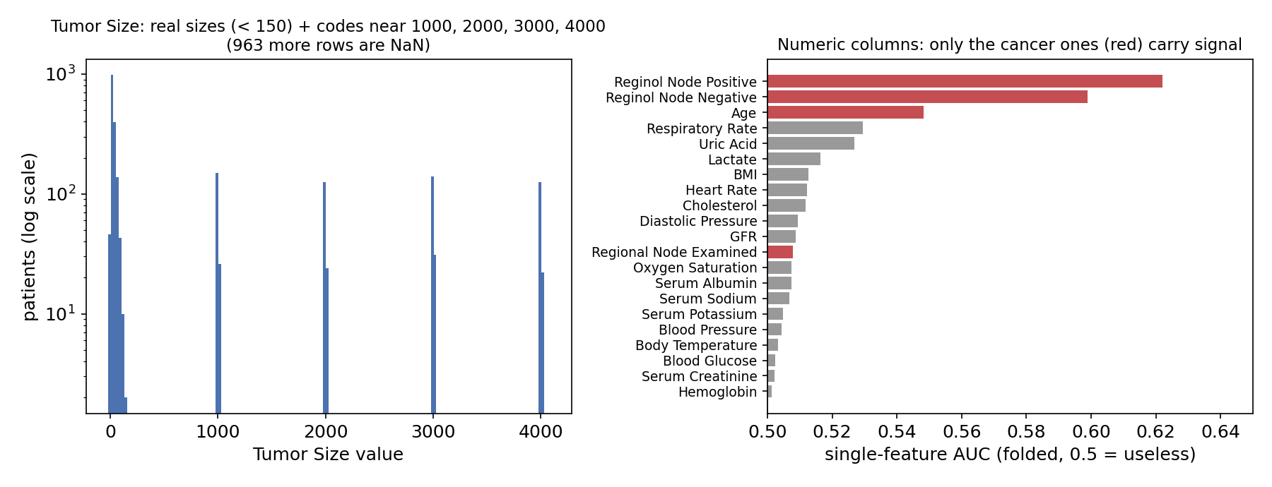
The death rate itself climbs exactly as oncology predicts: 10 % for T1 tumours against 37 % for T4, 10 % for N1 against 37 % for N3, 39 % when the cancer has spread (A Stage = Distant) and 41 % when both hormone receptors are negative. These staging variables are what a model should use.

The warm-up subtasks

Each one is a single line of pandas, but each hides a trap worth noticing.

1. Kidney function. Normal if GFR $\ge 90$, otherwise Mildly Decreased. Every test GFR is at least 60.1, so the two categories cover the whole test set (420 patients are Normal).
2. Creatinine risk. Compute the quartiles on the training set, not on the test set: $Q_1 = -2.454$, $Q_2 = 0.874$, $Q_3 = 4.397$ (pandas and numpy agree; with 3,219 values the interpolation convention changes nothing). Then use the inequalities exactly as given, with $\le$ on the upper bound of each band.
3. BMI flag. The statement first says "compute the mean BMI", then asks whether each BMI is strictly above the median. On the training set the mean is 29.115 and the median 29.199, and exactly 3 test patients fall between them, so the choice matters for 3 rows out of 805. The comparison sentence, which is the rule actually applied, names the median, so we use it.
4. Same T stage. Map each test patient's T stage to its count in the training set: T1 = 1281, T2 = 1430, T3 = 418, T4 = 90.

A first baseline

Encode the staging variables as numbers (T, N, 6th stage and grade as ordinal integers, distant spread and receptor status as 0/1, age, node counts, the cleaned size, race and marital status as one-hot columns), standardise, and fit a logistic regression. Predict Dead when $P(\text{Dead}) \ge 0.5$, the default of every classifier.

Averaged over three repetitions of 5-fold cross-validation, this model reaches an AUC of 0.739 and a precision of 0.574 on the Dead class, while flagging 108 of the 3,219 training patients (3.4 %, against a true death rate of 15.4 %).

Adding the seventeen clinical columns lowers the AUC to 0.728 and the precision to 0.546. Random forests (AUC 0.711) and gradient boosting (0.714) do worse than the linear model: with mostly ordinal staging variables and a weak signal, a smooth additive score is exactly the right shape, and flexible models only fit the noise.

The key idea

A probabilistic classifier does not output a class, it outputs a score $p(x)$, and the threshold $t$ is yours to choose. The default $t = 0.5$ maximises accuracy only when both kinds of error cost the same. Here they do not: a missed death (false negative) costs nothing, a false alarm (false positive) lowers the score. Raising $t$ keeps only the patients the model is surest about, and the precision rises:

threshold	patients flagged in CV (of 3,219)	precision
0.30	388	0.433
0.50	108	0.574
0.60	49	0.653
0.65	32	0.719
0.70	18	0.778
0.80	5	0.800

So why not push $t$ to 0.95 and flag a single patient? Because the score is computed on only 805 test patients, and precision computed on $n$ flagged patients is an average of $n$ coin flips. Its standard deviation is about

$$\sqrt{\frac{\pi(1-\pi)}{n}},$$

where $\pi$ is the true precision at that threshold. With $\pi = 0.75$ and $n = 4$, that is 0.22: one unlucky patient moves you by 25 points of precision, and with a very high threshold there is even a real chance of flagging nobody at all (scored 0 by most implementations). We simulated this directly: draw 805 training patients at random, apply each threshold to their out-of-fold probabilities, and record the precision.

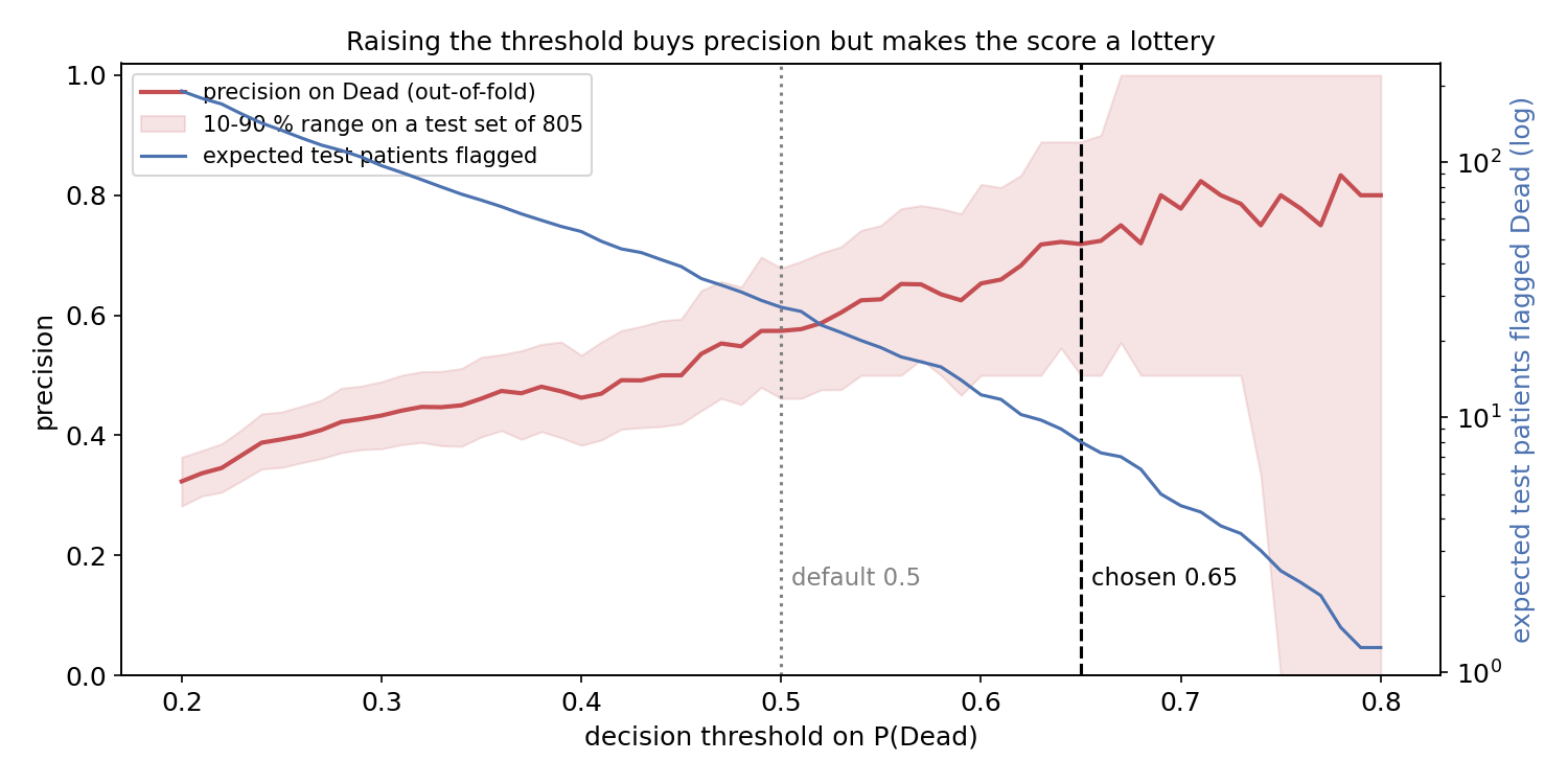
The figure shows the trade-off. Up to about $t = 0.65$ the mean precision rises and the worst case (10th percentile) stays at 0.50 or better. Beyond 0.70 the mean barely moves, but the band explodes: the expected number of flagged test patients drops below 5 and the score becomes a lottery. We choose $t = 0.65$: about 8 test patients flagged, an expected precision of 0.72 with a spread of $\pm 0.15$.

This is a general lesson about one-sided metrics. Precision alone, recall alone, or "accuracy on the positives" can each be pushed up by a degenerate strategy (predict almost nothing, or everything). Real metrics such as F1, average precision or precision at a fixed recall exist precisely to block that. Here the statement asks for precision, so the honest answer is to optimise precision and to say clearly what that does to the predictions: our model would be useless as a screening tool, since it would find only about 6 of the roughly 124 deaths in the test set.

The full solution

1. Subtasks 1 to 4: exact computations with training-set statistics, as described above.
2. Clean the features. Fill 6th Stage with IIA (always correct here), set Tumor Size codes above 500 to missing and fill with the median, encode stages ordinally, add the share of positive nodes, drop the seventeen clinical columns.
3. Model. Standardised logistic regression, $C = 0.3$ (the regularisation strength barely matters: AUC 0.738 to 0.740 for $C$ from 0.01 to 3).
4. Threshold. Choose $t$ on out-of-fold probabilities from repeated 5-fold CV, never on the test set; refit on all training data and flag test patients with $p \ge 0.65$ (9 patients in our run).

model = make_pipeline(StandardScaler(), LogisticRegression(C=0.3, max_iter=2000))
oof = cross_val_predict(model, X, y, cv=StratifiedKFold(5, shuffle=True), method="predict_proba")[:, 1]
model.fit(X, y)
t5 = np.where(model.predict_proba(X_test)[:, 1] >= 0.65, "Dead", "Alive")

Results

Subtask 5, cross-validated on the training set (the test labels are private):

approach	AUC	precision on Dead	flagged
sample output (everything Alive)		0 (5 points by rule)	0
random forest, threshold 0.5	0.711	0.538	52
gradient boosting, threshold 0.5	0.714	0.519	104
logistic regression + 17 clinical columns, 0.5	0.728	0.546	119
logistic regression, staging features, 0.5	0.739	0.574	108
same, threshold 0.60	0.739	0.653	49
same, threshold 0.65 (final)	0.739	0.719	32
same, threshold 0.80 (too few predictions, unstable)	0.739	0.800	5

At $60 \times$ precision, the final choice is worth about 43 of the 60 points in expectation, against about 34 for the default threshold. Subtasks 1 to 4 are deterministic and should earn their full 40 points, with the caveat that subtask 3 depends on reading "median" (3 rows would change with the mean).

What to remember

• Read the metric before choosing the model. A score that ignores false negatives turns the decision threshold into the main hyperparameter; the model itself barely changed between our variants.
• Choose thresholds on out-of-fold predictions, and think about the size of the test set. A metric averaged over few predictions has a large variance, $\sqrt{\pi(1-\pi)/n}$; simulating test-sized samples shows where optimising the mean starts to cost you in the worst case.
• Look for disguised missing values. Codes like 1000, 2000, 3000 in a size column, or a missing stage that the other columns determine exactly, are found by histograms and cross-tabulations, not by the model.
• Many columns do not mean much signal. Seventeen synthetic vital signs with AUC 0.5 only add variance; the simple, well-encoded staging variables carry the whole prediction, and a linear model on them beats forests and boosting.