Theory Test (17 problems)

The problem in brief

This is the written theory paper of the June 2025 training camp of the Romanian national AI team. It has 17 short problems that sweep the whole classical AI syllabus: data preparation (scaling, outliers, encoding, regularisation), probabilistic and tree classifiers, k-means, game search (minimax and alpha-beta), heuristic search (A*), logic and resolution, constraint satisfaction, approximate Q-learning, evaluation metrics, kernels and recommender systems. Each problem is a small hand computation followed by a "why" question. The paper is in Romanian; the answers below are our own derivations, and every number was rechecked with a short Python script (solution.py).

How you are scored

The paper is marked by hand. The published PDF gives no point scale and no answer key, so there is no threshold to compare with. What a marker looks for is visible in the wording: a correct number and a justification (several sub-questions say "Argumentați", "justify", and Problem 10 explicitly gives no credit to a proof that does not use resolution). The corrections below therefore always show the reasoning, not just the result.

Question by question

Problem 1: scaling and outliers

The table has a monthly income in euros (1 000 to 12 000) and a satisfaction score from 0 to 10.

a) A distance such as $\sqrt{(\Delta \text{income})^2 + (\Delta \text{score})^2}$ adds the two columns as if they had the same unit. A difference of 1 000 euros then counts a million times more than a difference of 1 point of satisfaction, so k-NN effectively ignores the score. Normalising puts both columns on a comparable scale, for example min-max scaling $x' = (x - \min)/(\max - \min)$ or standardisation $x' = (x - \mu)/\sigma$.

b) Sorted incomes: $1000, 2300, 3100, 4500, 5000, 12000$. With the "median of each half" rule, $Q_1 = 2300$ and $Q_3 = 5000$, so $\text{IQR} = 2700$ and the fences are

$$Q_1 - 1.5\,\text{IQR} = -1750, \qquad Q_3 + 1.5\,\text{IQR} = 9050 .$$

12 000 is the only outlier. Other quartile conventions move the fences a little (NumPy's linear interpolation gives $Q_1 = 2500$, $Q_3 = 4875$ and an upper fence of 8 437.5), but the verdict does not change.

c) Robust scaling, $x' = (x - \text{median})/\text{IQR}$. Standard scaling uses the mean and the standard deviation, which the 12 000 inflates: the mean jumps to 4 650 and the five ordinary users get squeezed together. The median and the IQR barely notice one extreme value.

Problem 2: encoding categories

a) CategorieAliment (dairy, meat, vegetables) is nominal: there is no natural order. Use one-hot encoding (three 0/1 columns). Mapping the categories to 0, 1, 2 would invent an order and distances (meat "between" dairy and vegetables) that a model would take seriously. ConținutGrăsime (low, medium, high) is ordinal, so ordinal encoding low = 0, medium = 1, high = 2 keeps the information that high > medium > low in a single column.

b) Min-max with $\min = 3.5$ and $\max = 13.5$, so a range of 10:

ID	price	scaled
1	5.4	0.19
2	13.5	1.00
3	3.8	0.03
4	11.0	0.75
5	3.5	0.00

Problem 3: L1 or L2?

The L2 penalty $\lambda \sum_j w_j^2$ has gradient $2\lambda w_j$, which shrinks every coefficient proportionally and never quite reaches zero. The L1 penalty $\lambda \sum_j |w_j|$ pushes every nonzero coefficient with the same force $\lambda$, so small coefficients hit exactly zero.

• a) many correlated features, shrink them without removing them: L2 (Ridge);
• b) remove irrelevant features, automatic selection: L1 (Lasso);
• c) only a small subset of features matters (a sparse truth): L1 (Lasso);
• d) a penalty spread evenly over all coefficients: L2 (Ridge).

Problem 4: Naive Bayes for Josh

Josh is absent on days 1 to 4 and present on days 5 to 10.

a) Counting (maximum likelihood estimation):

	$Y=0$ (4 days)	$Y=1$ (6 days)
$P(Y)$	0.4	0.6
$P(X_c = 1 \mid Y)$	0/4 = 0	3/6 = 1/2
$P(X_m = 1 \mid Y)$	0/4 = 0	2/6 = 1/3
$P(X_p = 1 \mid Y)$	2/4 = 1/2	4/6 = 2/3

(The probabilities for value 0 are the complements.)

b) For $X_c = 0, X_m = 0, X_p = 1$:

$$P(Y{=}0)\,P(x \mid Y{=}0) = 0.4 \cdot 1 \cdot 1 \cdot \tfrac12 = 0.200 ,$$ $$P(Y{=}1)\,P(x \mid Y{=}1) = 0.6 \cdot \tfrac12 \cdot \tfrac23 \cdot \tfrac23 \approx 0.133 .$$

Absent is more likely: after normalising, $P(Y{=}1 \mid x) = 0.133/0.333 = 0.4$.

c) With $k = 1$ and $V = 2$ values per sensor, every count gets $+1$ and every denominator $+2$:

	$Y=0$	$Y=1$
$P(X_c = 1 \mid Y)$	1/6	4/8 = 1/2
$P(X_m = 1 \mid Y)$	1/6	3/8
$P(X_p = 1 \mid Y)$	3/6 = 1/2	5/8

The main change is that no probability is 0 any more. Under MLE, a single pressure or motion reading would force $P(Y{=}0 \mid x) = 0$, whatever the other sensors say, which is far too confident after only 4 absent days. For the new observation, $0.4 \cdot \frac56 \cdot \frac56 \cdot \frac12 \approx 0.139$ against $0.6 \cdot \frac12 \cdot \frac58 \cdot \frac58 \approx 0.117$: the decision is still absent, but less clearly ($P(Y{=}1 \mid x) \approx 0.46$). Smoothing the prior as well, $(4+1)/12$ and $(6+1)/12$, gives the same decision.

Problem 5: a decision tree for the exam

The six students: 4 passed, 2 failed.

a) $E(\text{Examen}) = -\frac23 \log_2 \frac23 - \frac13 \log_2 \frac13 = \log_2 3 - \frac23 \approx 1.58 - 0.67 = 0.92$ bits.

b) For each value of Parcurs: "small" has 1 pass and 1 fail (entropy 1), "medium" also (entropy 1), "large" has 2 passes (entropy 0). Each value covers a third of the students:

$$E(\text{Examen} \mid \text{Parcurs}) = \tfrac13 \cdot 1 + \tfrac13 \cdot 1 + \tfrac13 \cdot 0 = \tfrac23 \approx 0.67 .$$

c) To build the tree, compare with the other attribute. The students who studied all passed (entropy 0). Those who did not have 2 fails and 1 pass (entropy 0.92). So $E(\text{Examen} \mid \text{Învățat}) = \frac12 \cdot 0.92 = 0.46$. The information gains are $0.92 - 0.67 = 0.25$ for Parcurs and $0.92 - 0.46 = 0.46$ for Învățat, so the root tests "studied?":

• studied = yes: passed (3 of 3);
• studied = no: test Parcurs: small gives failed, medium gives failed, large gives passed.

Every leaf is pure: the tree fits the six students exactly with 4 leaves.

Problem 6: one k-means step with Manhattan distance

Distances to $C_1 = (2,2)$ and $C_2 = (8,9)$:

point	to $C_1$	to $C_2$	cluster
A(1,2)	1	14	1
B(2,1)	1	14	1
C(4,5)	5	8	1
D(7,8)	11	2	2
E(8,8)	12	1	2
F(9,9)	14	1	2

b) New centroids (coordinate-wise means):

$$C_1 = \left(\tfrac{1+2+4}{3}, \tfrac{2+1+5}{3}\right) = (2.33,\ 2.67), \qquad C_2 = \left(8,\ \tfrac{25}{3}\right) = (8,\ 8.33).$$

(With the Manhattan distance, the centre that minimises the sum of distances would be the coordinate-wise median, as in k-medians. The statement asks for the mean, so we use the mean.)

Problem 7: minimax and alpha-beta

a) Each MAX node on the third level takes the largest of its three leaves, each MIN node the smallest of those, and the root the largest MIN value:

• MIN 1: $\min(5, 9, 7) = 5$;
• MIN 2: $\min(10, 6, 9) = 6$;
• MIN 3: $\min(7, 7, 9) = 7$.

The root is worth 7. MAX plays the third branch, MIN answers with its first child (worth 7, ties broken to the left), and the game ends on the leaf 7 (the middle leaf of 3, 7, 2).

b) Yes, cuts happen. Going left to right and cutting when $v \ge \beta$ at a MAX node or $v \le \alpha$ at a MIN node:

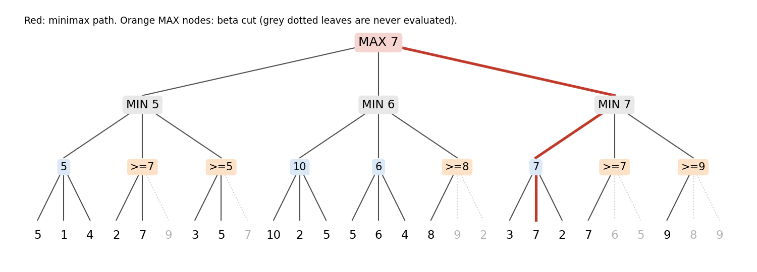
1. Under MIN 1, after the first MAX child, $\beta = 5$. The second MAX child sees 2, then 7: since $7 \ge 5$, MIN will never let play reach it, and leaf 9 is pruned (beta cut).
2. Third MAX child of MIN 1: 3, then 5, and $5 \ge \beta = 5$: leaf 7 is pruned (beta cut, on equality).
3. At the root, $\alpha = 5$. Under MIN 2, $\beta$ goes to 10, then 6. The third MAX child sees 8, and $8 \ge 6$: leaves 9 and 2 are pruned.
4. Now $\alpha = 6$. Under MIN 3, the first MAX child is worth 7, so $\beta = 7$. The second sees 7, and $7 \ge 7$: leaves 6 and 5 are pruned.
5. The third sees 9, and $9 \ge 7$: leaves 8 and 9 are pruned.

All five are beta cuts (at MAX nodes, because the MIN parent already has something better). There is no alpha cut: the MIN values come in increasing order (5, 6, 7), so no MIN node ever falls below the current $\alpha$. Alpha-beta evaluates 19 leaves instead of 27 and still returns 7. If your course only cuts on strict inequality, cuts 2 and 4 disappear and 22 leaves are evaluated.

c) If MAX takes control of a MIN node, that node gives MAX the largest of its children, minus the cost: $9 - 2 = 7$ for MIN 1, $10 - 2 = 8$ for MIN 2 and $9 - 2 = 7$ for MIN 3. Forcing MIN 2 to enter the subtree worth 10 gives 8 > 7, so using the ability is optimal, on the second branch. (Paying for it on the third branch would only tie with the free value 7.)

Problem 8: A* and heuristics

Edges: G-F 5, F-D 3, G-D 9, G-E 2, E-D 8, D-B 5, B-A 1, D-C 3, C-B 1, C-A 4. True distances to G (Dijkstra from G): $h^*(G)=0$, $h^*(E)=2$, $h^*(F)=5$, $h^*(D)=8$, $h^*(C)=11$, $h^*(B)=12$, $h^*(A)=13$.

a) Admissible means $h(s) \le h^*(s)$ for every state. The given values all satisfy it ($10 \le 13$, $9 \le 11$, $7 \le 8$, $1.5 \le 2$, $4.5 \le 5$), so $h$ is admissible if and only if $\mathbf{0 \le h(B) \le 12}$.

Consistent means $h(u) \le c(u,v) + h(v)$ for every edge, in both directions (the graph is undirected), with $h(G) = 0$. The edges that do not touch B are fine (for example $h(D) = 7 \le 3 + 4.5$). The edges at B give:

• B-A, cost 1: $|h(B) - 10| \le 1$, so $9 \le h(B) \le 11$;
• B-C, cost 1: $|h(B) - 9| \le 1$, so $8 \le h(B) \le 10$;
• B-D, cost 5: $|h(B) - 7| \le 5$, so $2 \le h(B) \le 12$.

So $h$ is consistent if and only if $\mathbf{9 \le h(B) \le 10}$. As expected, it is a narrower window than admissibility, since consistency implies admissibility.

b) Careful: as a returned path, A → C → B → D → E → G is impossible for graph-search A*, whatever the heuristic. A is expanded first and puts B in the frontier with $g = 1$; later, reaching B through C would cost $g = 5$, which never replaces the better parent A. The question therefore makes sense as the order of expansion. We need, step by step:

1. after A: $f(C) = 4 + h(C) < f(B) = 1 + h(B)$;
2. after C (D now has $g = 7$): $1 + h(B) < 7 + h(D)$;
3. B lowers D to $g = 6$, then D is expanded and puts F ($g = 9$), E ($g = 14$) and G ($g = 15$) in the frontier: we need $14 + h(E) < 9 + h(F)$ and $14 + h(E) < 15$;
4. finally G (15) must come out before F: $15 < 9 + h(F)$.

$h = (A{:}10,\ B{:}5,\ C{:}0,\ D{:}0,\ E{:}0,\ F{:}10,\ G{:}0)$ satisfies all of these, and a simulation confirms the expansion order A, C, B, D, E, G. This $h$ is not admissible ($h(F) = 10 > 5$), and it has to be inadmissible: E is expanded before F although F is on the optimal route. A* then returns the path A → B → D → G of cost 15 instead of the optimal 13, which illustrates what an overestimating heuristic does.

c) Yes: $g(s) = \max(h_1(s), h_2(s))$. It is admissible because each of the two is at most $h^*(s)$, so their maximum is too. It dominates both ($g \ge h_1$ and $g \ge h_2$ everywhere), and a dominating admissible heuristic never makes A* expand more nodes (for consistent heuristics, every node expanded with $g$ is also expanded with $h_1$ and with $h_2$). On our graph, with $h_1 = h$ from a) and $h_2(s) =$ "smallest edge leaving $s$" (1 for A, 1 for B, 1 for C, 3 for D, 2 for E, 3 for F, 0 for G), $g$ takes $h_1$ almost everywhere but improves E to 2. By contrast, $h_1 + h_2$ is not a safe choice: it can overestimate.

Problem 9: propositional resolution

a) Let $P$ = "PROG1 is correct" and $Q$ = "PROG1 produces conforming results". The premises are $P \to Q$ and $P$, and the conclusion is $Q$.

b) Put everything in CNF and add the negation of the conclusion:

$$(1)\ \neg P \lor Q \qquad (2)\ P \qquad (3)\ \neg Q .$$

Resolving (1) with (3) on $Q$ gives (4) $\neg P$. Resolving (4) with (2) gives the empty clause $\square$. The premises plus $\neg Q$ are contradictory, so $Q$ follows: this is modus ponens, proved by refutation.

Problem 10: first-order resolution

a) With $Plecat(x)$ = "the head of $x$ is bowed" and $Taiat(x)$ = "the head of $x$ is cut by the sword", the proverb "a bowed head is not cut by the sword" becomes

$$\forall x\ \big(Plecat(x) \to \neg Taiat(x)\big), \qquad \text{plus the fact } Taiat(Marcel).$$

The goal is $\neg Plecat(Marcel)$.

b) Clauses: (1) $\neg Plecat(x) \lor \neg Taiat(x)$, (2) $Taiat(Marcel)$, (3) the negated goal $Plecat(Marcel)$. Resolve (1) and (3) with the unifier $\{x / Marcel\}$, which gives (4) $\neg Taiat(Marcel)$. Resolve (4) with (2), which gives $\square$. Hence Marcel's head was not bowed. (The logic is the contrapositive: no bowed head is cut, Marcel's head was cut, so it was not bowed.)

Problem 11: arc consistency (AC-3)

Domains $X \in \{1..10\}$, $Y \in \{5..10\}$, $Z \in \{5..15\}$. Constraints $X > Y$, $Y + Z = 12$, $X + Z = 15$.

a) An arc $X \to Z$ is consistent if every value of $X$ has a supporting value of $Z$. Checking the six arcs:

• $X \to Y$: no ($x \le 5$ has no smaller $y$);
• $Y \to X$: no ($y = 10$ would need $x = 11$);
• $Y \to Z$: no ($y = 8$ needs $z = 4$);
• $Z \to Y$: no ($z = 8$ needs $y = 4$);
• $Z \to X$: no ($z = 15$ needs $x = 0$);
• $X \to Z$: yes, since every $x \in \{1..10\}$ has $z = 15 - x \in \{5..14\}$.

So exactly one arc, $X \to Z$, is already arc-consistent.

b) The queue starts with all arcs, in both directions: 3 binary constraints give 6 arcs. An arc $(X_k, X_i)$ is put back into the queue only when a value is deleted from the domain of $X_i$. A domain of size $d$ can lose at most $d$ values, so each arc enters the queue at most $d$ times, where $d$ is the largest domain size: here $d = 11$ (the domain of $Z$). This is what gives AC-3 its $O(c\,d^3)$ running time for $c$ constraints.

c) Running AC-3:

1. $Y \to Z$ with $Y + Z = 12$: $Y \in \{5,6,7\}$;
2. $Z \to Y$: $Z \in \{5,6,7\}$;
3. $X \to Z$ with $X + Z = 15$: $X \in \{8,9,10\}$;
4. $X > Y$ now holds for every pair ($8 > 7$), and all the other arcs are consistent.

Final domains: $X \in \{8,9,10\}$, $Y \in \{5,6,7\}$, $Z \in \{5,6,7\}$. Note that arc consistency does not solve the problem by itself: the real solutions are only the three triples $(X,Y,Z) = (y+3,\ y,\ 12-y)$ for $y \in \{5,6,7\}$.

Problem 12: scheduling as a CSP

a) One variable per exam, $M$ (Math), $C$ (CS) and $P$ (Physics). Each takes a value that is a (room, slot) pair, with domain $\{S1, S2\} \times \{T1, T2, T3\}$, 6 values. Write $room(\cdot)$ and $time(\cdot)$ for the two parts of a value.

b) The constraints:

• $time(M) \neq time(C)$ (shared students);
• $room(P) \neq room(C)$;
• a room hosts at most one exam per slot: $M \neq C$, $M \neq P$ and $C \neq P$ as pairs (all-different on the (room, slot) values).

c) Backtracking in the order $M, C, P$, values in lexicographic order:

1. $M = (S1, T1)$;
2. $C$: $(S1, T1)$ is rejected (same pair, and same slot as M); $(S1, T2)$ is accepted;
3. $P$: $(S1, \cdot)$ is rejected (same room as C); $(S2, T1)$ is accepted (it differs from M's pair, and from C's room).

Solution: Math in S1 at T1, CS in S1 at T2, Physics in S2 at T1. No backtrack was even needed.

Problem 13: approximate Q-learning for Pacman

In the figure, Pacman sits between two ghosts (one directly to its left, one directly to its right), with a food pellet directly above. The wall below makes "down" impossible. In the current state, $A(s) = 2$ (two adjacent ghosts) and $D(s) = 1$ (one adjacent pellet).

a) The features for each action:

action	$B$ (ghosts hit)	$C$ (ghosts adjacent after)	$F_g = A+B+C$	$E$ (food eaten)	$F_p = D + 2E$
left	1	0	3	0	1
right	1	0	3	0	1
up	0	0	2	1	3
stay	0	2	4	0	1

After "left", Pacman is on the ghost (distance 0, counted in $B$), and the other ghost is now 2 cells away, so $C = 0$. After "up", both ghosts are diagonal, at Manhattan distance 2, so $C = 0$.

b) With $Q = -10\,F_g + 100\,F_p$: $Q(\text{left}) = Q(\text{right}) = -30 + 100 = 70$, $Q(\text{up}) = -20 + 300 = \mathbf{280}$, $Q(\text{stay}) = -40 + 100 = 60$. "Up" is the best action.

c) In $s'$ (the pellet's cell), no ghost and no pellet is adjacent, so $A(s') = D(s') = 0$. "Down" goes back between the ghosts: $F_g = 0 + 0 + 2 = 2$, $F_p = 0$, so $Q = -20$. "Stay" gives $Q = 0$. Then

$$Q_{\text{new}}(s, \text{up}) = 250 + 0.5 \cdot \max(-20, 0) = 250 .$$

d) The error is $\delta = 250 - 280 = -30$, and the features of "up" are $F_g = 2$, $F_p = 3$:

$$w_g = -10 + 0.5 \cdot (-30) \cdot 2 = -40, \qquad w_p = 100 + 0.5 \cdot (-30) \cdot 3 = 55 .$$

The prediction was too optimistic, so both weights move in the direction that lowers $Q(s, \text{up})$. The food weight drops a lot (Pacman had overrated food), and the ghost weight becomes more negative (ghosts now look more dangerous).

Problem 14: metrics from a confusion matrix

Rows are true classes, columns predictions. Column sums: 46, 48, 56. Row sums: 50 each.

a) Precision: $P_A = 40/46 = 0.870$, $P_B = 35/48 = 0.729$, $P_C = 40/56 = 0.714$.

b) Recalls are $0.8$, $0.7$ and $0.8$, so

$$F1_A = 0.833, \quad F1_B = 0.714, \quad F1_C = 0.755, \qquad \text{macro-}F1 = 0.767 .$$

c) Micro-averaged recall pools all the classes: $\frac{40 + 35 + 40}{150} = 0.767$. (In single-label classification, micro recall always equals accuracy.)

d) If missing a class-C case is very costly (a rare, serious disease), maximise the recall of class C (sensitivity), possibly under a minimum-precision constraint, or use $F_\beta$ with $\beta > 1$. Ways to get there: lower the decision threshold for C (predict C as soon as $P(C \mid x)$ exceeds, say, 0.2), weight class C more in the loss (cost-sensitive learning), or rebalance the training data (oversampling C, SMOTE). Here 11 of the 50 B cases are predicted as C and 8 of the 50 C cases as B, so the B/C boundary is where to work.

Problem 15: a kernel and a non-kernel

a) There are finitely many possible 16×16 patches: $N = 256^{256}$ of them. Index them $p_1, \dots, p_N$, and define $\varphi(x) \in \{0,1\}^N$ by $\varphi_i(x) = 1$ if patch $p_i$ appears somewhere in $x$, and 0 otherwise. Then

$$\varphi(x) \cdot \varphi(x') = \sum_{i=1}^{N} \varphi_i(x)\,\varphi_i(x') = \#\{i : p_i \text{ appears in both}\} = k_1(x, x') .$$

So $k_1$ is an inner product in $\mathbb{R}^d$ with $d = 256^{256} \in \mathbb{N}^*$, which makes it a kernel. The "count once" rule in the statement is exactly what makes the coordinates 0/1. An image smaller than 16×16 simply maps to the zero vector.

b) Take three images:

• $x_1$: a 16×16 all-black square (patch $a$);
• $x_3$: a 16×16 all-white square (patch $b$);
• $x_2$: a 16×32 image, black on the left half and white on the right half, which contains both $a$ and $b$.

$x_1$ and $x_3$ share no patch, and each image shares a patch with itself, so

$$G = \begin{pmatrix} 1 & 1 & 0 \\ 1 & 1 & 1 \\ 0 & 1 & 1 \end{pmatrix}, \qquad f = \begin{pmatrix} 1 \\ -1 \\ 1 \end{pmatrix}.$$

Then $f^\top G f = (1 + 1 + 1) + 2(-1 + 0 - 1) = -1 < 0$, so $G$ is not positive semidefinite (its eigenvalues are $1-\sqrt2$, $1$ and $1+\sqrt2$), and $k_2$ is not a kernel. The intuition: "share at least one patch" is not transitive. $x_1 \sim x_2$ and $x_2 \sim x_3$ but $x_1 \not\sim x_3$, and no inner product of feature vectors can behave like that with these 0/1 values.

Problem 16: user-based collaborative filtering

Means over each user's own ratings: $\bar R_{u_1} = \frac{5+3+1}{3} = 3$, $\bar R_{u_2} = \frac{4+3+2}{3} = 3$, $\bar R_{u_3} = \frac{1+1+5+5}{4} = 3$.

a)

• $u_1, u_2$ share items 1 and 4. The deviations are $(2, -2)$ and $(1, -1)$, so $\text{sim} = \frac{2 + 2}{\sqrt{8}\,\sqrt{2}} = \mathbf{1}$.
• $u_1, u_3$ share items 1, 2 and 4. The deviations are $(2, 0, -2)$ and $(-2, -2, 2)$, so $\text{sim} = \frac{-4 + 0 - 4}{\sqrt{8}\,\sqrt{12}} = \frac{-8}{4\sqrt6} = -\frac{2}{\sqrt6} \approx \mathbf{-0.82}$.

$u_2$ is the most similar to $u_1$ (perfect agreement), while $u_3$ has opposite tastes.

b)

$$\hat R_{u_1,3} = 3 + \frac{1\cdot(3-3) + (-0.82)(5-3)}{1 + 0.82} = 3 - \frac{1.63}{1.82} \approx 2.10 .$$

The negative similarity is used constructively: $u_3$ loved item 3, and since $u_3$ is an "anti-$u_1$", that pulls the prediction below $u_1$'s mean. (If you compute each mean only over the co-rated items, you get slightly different numbers. Say which convention you use.)

c) A new user has no ratings, so no co-rated items, so every similarity is undefined and the formula collapses (cold start). A content-based fallback: describe each item by a feature vector $c_j$ (for example genres as 0/1). Ask the new user for a few liked genres at sign-up, or use the first items they click, to build a profile vector $p_u$ (the average of the liked items' vectors). Then recommend the items with the highest $\cos(p_u, c_j)$. It needs no other user, so it works from the first interaction, and you can switch progressively to collaborative filtering as ratings accumulate (a hybrid system).

Problem 17: the PQ kernel is an inner product

Index the coordinates of a feature vector by the pairs $i < j$, so the vector has $\binom{n}{2}$ coordinates, and set

$$\Psi_{ij}(x) = \operatorname{sign}(x_i - x_j) \in \{-1, +1\}.$$

(For a permutation there are no ties, so the sign is never 0.) Then

$$\langle \Psi(x), \Psi(y) \rangle = \sum_{i<j} \operatorname{sign}(x_i - x_j)\,\operatorname{sign}(y_i - y_j).$$

Each term is $+1$ exactly when $(x_i - x_j)(y_i - y_j) > 0$ (a concordant pair) and $-1$ exactly when it is $< 0$ (a discordant pair). The sum is therefore $P - Q = k_{PQ}(x, y)$, an explicit inner product, so $k_{PQ}$ is a kernel. (We checked the identity on random permutations.) Dividing by $\binom{n}{2}$ gives Kendall's $\tau$, which shows that Kendall's correlation is a normalised kernel. For rankings with ties, the same $\Psi$ gives 0 on tied pairs, which matches the definitions of $P$ and $Q$.

What to remember

• Scale-sensitive models need scaling, and outliers decide which scaler. With distances (k-NN, k-means, SVM), unscaled columns silently drop out. With an outlier, use the median and the IQR, not the mean and the standard deviation.
• Search questions are bookkeeping: write the frontier. For alpha-beta, note $\alpha$ and $\beta$ at each node and check "$v \ge \beta$" or "$v \le \alpha$". For A*, write $f = g + h$ at each step. Before designing a heuristic, ask whether the requested behaviour is even reachable: in Problem 8, no heuristic can make A* return a path through a worse parent.
• Admissible means never overestimating; consistent is a triangle inequality on every edge. The max of admissible heuristics is admissible and dominates both.
• To prove a kernel, exhibit the feature map; to disprove it, exhibit a Gram matrix with $f^\top G f < 0$. Three well-chosen points usually suffice, and a non-transitive similarity is the classic counterexample.
• Approximate Q-learning is linear regression on the TD target. $\delta = (r + \gamma \max_{a'} Q(s', a')) - Q(s, a)$, then $w_i \mathrel{+}= \alpha\,\delta\,F_i$: each weight moves in proportion to how active its feature was.