The Ghost in the Machine

The problem in brief

You monitor 200 cloud servers. Each row is one snapshot of one server: six sensor metrics (CPU, memory, disk I/O, latency, error rate, temperature), plus an undocumented health_score, the server's region and hardware type, a short alert title written by humans in many styles, and a multi-line system log. From one training day (6 000 rows) you must predict, for a test day two weeks later (1 500 rows): (A) whether the server will fail in the next 4 hours, where the label is missing for 40 % of training rows, and (B) an anomaly_score between 0 and 100. The data is deliberately messy: missing values, impossible negative readings, free-form text.

The test labels are private. We validate on the last six hours of the training day (training on 00:00-17:59, scoring 18:00-23:59), which is the closest we can get to "a later period".

How you are scored

Two tasks, 50 points each:

$$\text{A: } 50\cdot\operatorname{clip}\!\Big(\frac{F_1-0.3}{0.3},\,0,\,1\Big), \qquad \text{B: } 50\cdot\operatorname{clip}\!\Big(\frac{13-\text{MAE}}{5},\,0,\,1\Big).$$

$F_1$ is computed on the positive class (failure = 1), and the answers must be exactly 0 or 1. Full marks need $F_1 \ge 0.6$ and $\text{MAE} \le 8$. Below $F_1=0.3$ or above $\text{MAE}=13$, the task scores zero.

First look at the data

• Failures are rare: 19.6 % of the labelled rows. Predicting "fails" everywhere already gives $F_1 = 0.32$, so the scale really starts at 0.3.
• Corrupted sensors: about 5 % of each metric is missing, and some disk I/O and error-rate values are negative, which is physically impossible. We treat them as missing and keep a flag.
• The text is very structured underneath. The 60-odd alert titles reduce to a few families once the server name is removed: six "routine" phrasings ("Heartbeat OK", "Scheduled health check"...) and alerts about errors, memory, CPU, network or disk. The logs contain only 33 distinct message templates once digits are masked, in five severity levels from DEBUG to CRIT. Some templates are strong failure signals: OOM killer, ECC memory errors, RAID degraded, cascading service failures.
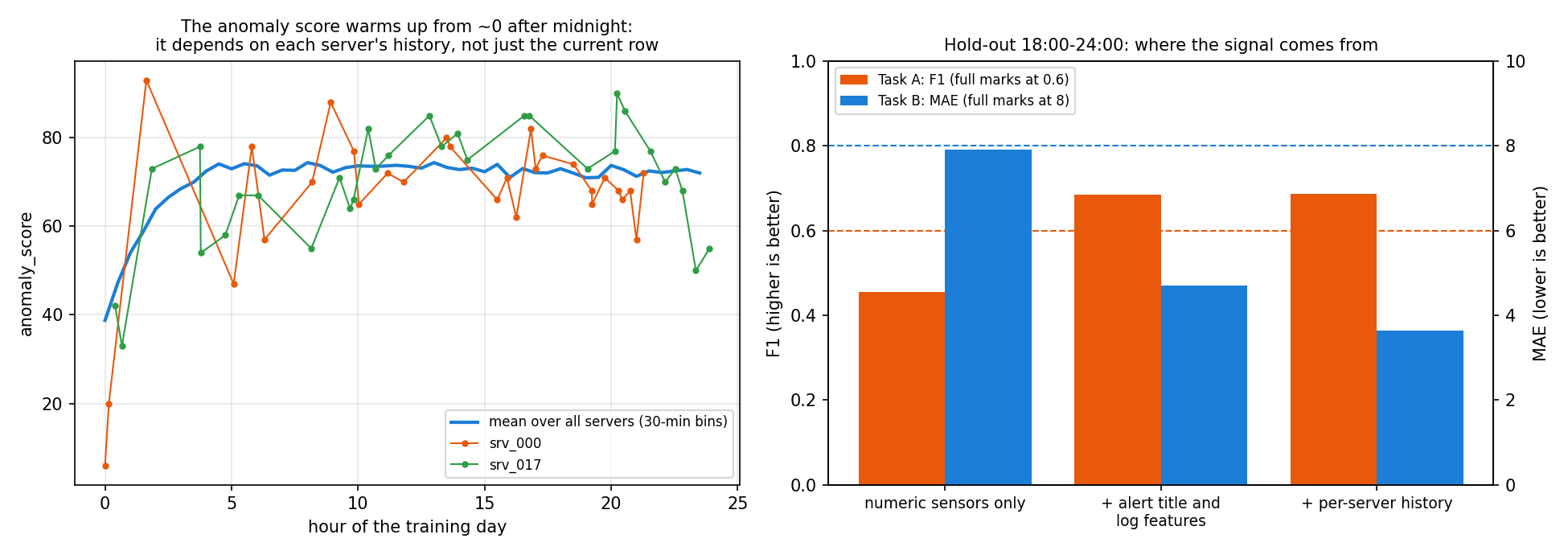
• The anomaly score has a memory. Averaged over servers, it is about 40 just after midnight and climbs to a plateau of 73 by 04:00. The first snapshot of srv_000 scores 6 and the next one 20. A score that starts near 0 at the beginning of the recording and settles later behaves like a running statistic of each server's history, not a function of the current row alone. The test day also starts at 00:01, so the same warm-up applies there.

A first baseline

LightGBM on the six raw sensor metrics (plus health score) only:

• A: $F_1 = 0.454$, which is only 25 points;
• B: $\text{MAE} = 7.91$, barely under the full-marks line (predicting the median gives 8.89).

The numbers alone carry little signal. Most of the information is in the text.

The key idea

Turn the text into counts, and give each row its server's past.

1. Logs as counted events. For each row we count the lines of each severity level (DEBUG, INFO, WARN, ERROR, CRIT) and of each important template (OOM, ECC, RAID, cascade, thermal throttling, link flap, write failures...). We also parse the numbers the templates contain (GC pause in ms, health-check latency, connection-pool percentage, the cpu and mem values the log repeats) and add a single severity index $\text{sev}=\#\text{WARN}+3\,\#\text{ERROR}+9\,\#\text{CRIT}$. The alert title becomes a "routine" flag plus five subsystem flags. These counts raise $F_1$ from 0.45 to 0.68 and cut the MAE from 7.9 to 4.7.
2. Per-server history. Sort each server's rows by time and add: the row's position $k$ in the day (this is what captures the warm-up), the running mean and an exponentially weighted mean (half-life of 3 snapshots) of severity, error rate, CRIT count and the routine flag, the previous and next snapshot's values, and the minutes since the previous snapshot. If the anomaly score is a smoothed history, these features describe exactly that history. The MAE drops further, from 4.7 to 3.6. Failure prediction hardly moves: a failure in the next 4 hours depends mostly on what the server shows now.
3. The F1 threshold matters as much as the model. With 20 % positives, the threshold that maximises F1 is far below 0.5. We pick it from out-of-fold predictions on the training rows (it comes out around 0.18 to 0.20), never on the hold-out. At 0.5, the same model scores only about 0.60 on the hold-out.

The full solution

1. Cleaning: negative disk I/O and error rates become missing (with a flag), and we add the count of missing metrics per row.
2. Features (about 75 in total): metrics, region and type codes, hour, alert flags, log-level and template counts, parsed log numbers, the severity index, and the per-server history features.
3. Task A: LightGBM classifier on the 3 576 labelled rows (600 trees, 15 leaves, learning rate 0.03, row and column subsampling 0.8). The 0/1 threshold is chosen by 5-fold out-of-fold F1.
4. Task B: LightGBM with the L1 (absolute error) objective, which matches the MAE metric, trained on all 6 000 rows, since the anomaly score is never missing. Predictions are clipped to [0, 100].
5. For the submission, refit on the whole training day and write two rows per test id (subtaskID 1 and 2).

We also tried three ideas for task A that did not change anything beyond noise: using the predicted anomaly score as a feature (0.672), self-training on confident pseudo-labels for the unlabelled rows (0.695), and even the true anomaly score as a feature (0.689, an upper bound). The unlabelled 40 % carries little extra information here.

Results

Hold-out: last 6 hours of the training day (1 564 rows, 625 of them with a failure label).

features	A: F1	B: MAE	points (A + B)
always "failure" / predict the median	0.324	8.889	4 + 41
sensor metrics only	0.454	7.910	26 + 50
+ alert title and log features (single row)	0.684	4.698	50 + 50
+ per-server history	0.686	3.642	50 + 50
final solution.py (same features, fixed seed)	0.678	3.722	100
+ predicted anomaly score as an A feature	0.672
+ self-training on unlabelled rows	0.695

Both tasks clear their full-marks lines with room to spare ($F_1$ 0.68 against 0.6, MAE 3.7 against 8). The test day comes from another period, so the true margin will be smaller. The feature distributions of the two days are very close (mean severity 13.8 against 13.7, error rate 5.5 against 5.6), which is reassuring.

What to remember

• Semi-structured logs are a bag of events. Mask the variable parts (digits, ids), count the templates and severity levels, and parse the numbers they carry. Here that was worth more than all the sensors.
• Look at the target over time. A score that warms up from zero is a running statistic, and per-entity history features (cumulative mean, EWMA, previous and next values) are what model it.
• For F1 on an imbalanced class, tune the threshold, and tune it on out-of-fold predictions, never on the evaluation set. The optimum here is about 0.2, not 0.5.
• Match the training loss to the metric: L1 for MAE.
• Validate on a later period when the test set is a later period. A random split would mix neighbouring snapshots of the same server and flatter the model.