The problem in brief
Test vehicles carry gas, temperature and flame sensors that report once per second. Each reading of the training set (3,232 rows) is labelled NORMAL, GAS_LEAK, OVERHEAT or FIRE; the test set has 800 unlabelled readings. Besides the useful sensors (raw gas, temperature, flame, their moving averages, a drifting gas sensor, the ambient temperature) the table contains distractors: sensor noise, timestamp, battery level, speed, weather and sensor ID. About 28 % of every numeric value is missing. The task has four parts: describe the classes, compute a Mahalanobis anomaly score for each test reading, turn it into LOW/MEDIUM/HIGH risk levels, and build a 4-class classifier.
How you are scored
| subtask | what | points |
|---|---|---|
| 1 | 12 descriptive statistics, all must be right | 20 |
| 2 | Mahalanobis distance per test reading, proportional to the share within | 15 |
| 3 | risk level per test reading, proportional to the share correct | 15 |
| 4 | predicted hazard, weighted F1 | 50 |
Weighted F1 averages the per-class F1 scores with weights equal to the class frequencies :
Subtask 4 gives 50 points for , 0 below 0.60 and a linear interpolation in between (statement, "Evaluation"). Subtasks 1 to 3 are deterministic computations: what matters is following the recipe exactly. Test labels are private, so subtask 4 is evaluated by 5-fold cross-validation on the training set.
First look at the data
The four classes are perfectly balanced (about 800 readings each) and the physics is simple:
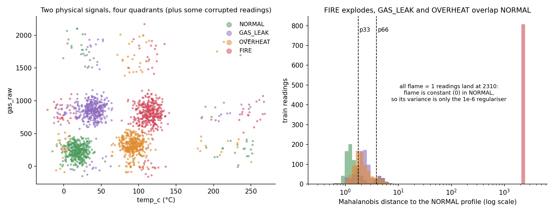
Two binary questions, "is it hot?" and "is there gas?", carve four quadrants, and the flame sensor fires for 807 of the 815 FIRE readings and never for the other classes. A few observations matter for what follows:
- Redundant sensors.
gas_sensor_driftis almost a copy ofgas_raw(correlation 0.97) andambient_tempoftemp_c(0.99). The moving averagesgas_avgandtemp_avgare much noisier versions (correlation 0.4 with the raw values). - Corrupted readings. About 4 % of readings have absurd values (gas near 2000, temperature above 180 °C) whatever their label.
- Distractor columns. Weather and sensor ID are spread evenly across classes; timestamp, noise, battery, speed and the rates
dGas,dTemphave Spearman correlations below 0.025 with the label.
Subtask 1: hazard profile
Straight pandas, with the default behaviour of skipping missing values in the means (temp_c and gas_raw are the "temperature" and "gas concentration" of the statement):
| NORMAL | GAS_LEAK | OVERHEAT | FIRE | |
|---|---|---|---|---|
| share of readings (%) | 25.12 | 24.94 | 24.72 | 25.22 |
mean temp_c (°C) | 28.5 | 46.9 | 93.0 | 112.0 |
mean gas_raw | 321.2 | 867.4 | 379.9 | 825.1 |
The table confirms the quadrant picture: OVERHEAT and FIRE are hot, GAS_LEAK and FIRE are gassy. (The NORMAL mean temperature, 28.5 °C, is above its median, 19.7 °C, because of the corrupted hot readings: the mean is sensitive to outliers.)
Subtask 2: the Mahalanobis anomaly score
Feature selection. Encode the label as NORMAL , GAS_LEAK , OVERHEAT , FIRE and rank the 13 numeric columns (all except id) by the absolute Spearman correlation with this code, computed on the available pairs:
| feature | temp_avg | flame | temp_c | ambient_temp | gas_avg | gas_sensor_drift | gas_raw | timestamp_ms |
|---|---|---|---|---|---|---|---|---|
| 0.778 | 0.772 | 0.759 | 0.749 | 0.378 | 0.361 | 0.359 | 0.023 |
The top 6 are temp_avg, flame, temp_c, ambient_temp, gas_avg, gas_sensor_drift. Reassuringly, computing Spearman after median imputation reorders them (flame moves first) but selects the same six, and there is no tie. Temperature features rank higher than gas features because the code is ordinal: temperature increases along 0, 1, 2, 3 except for one step, while gas goes low, high, low, high.
Preparation. Fill missing values with the train median of each column, then standardise with the train mean and standard deviation (StandardScaler convention, population standard deviation).
Distance. With and the mean and covariance (np.cov, denominator ) of the standardised NORMAL training rows,
Unlike the Euclidean distance, Mahalanobis measures each direction in units of the NORMAL spread along it, and it discounts correlated features: temp_c and ambient_temp are nearly the same measurement and should not count twice. Geometrically, it is the Euclidean distance after "whitening" the NORMAL cloud into a round ball.
The surprise: why every fire scores 2310. No NORMAL reading has flame = 1, so the flame column is constant inside NORMAL: its variance there is exactly 0 and is singular. The regulariser makes the matrix invertible, but along the flame direction the "allowed spread" is now . A reading with flame is standard deviations away from NORMAL on that axis (0.433 is the standard deviation of flame over the whole train), so its distance is about , whatever the other sensors say. That is visible as the lone red bar in the figure.
This has a practical consequence for the tolerance: for those readings, a tiny convention change (standard deviation with instead of , for instance) changes the third significant digit, about in absolute value, and fails the tolerance on about a quarter of the test set. We used the standard library conventions (StandardScaler then np.cov), and checked our formula against scipy.spatial.distance.mahalanobis.
The other surprise is in the opposite direction: GAS_LEAK and OVERHEAT readings get distances of only about 2.4, barely more than NORMAL (1.8). Two reasons. The NORMAL class contains the corrupted readings, which inflate its covariance: the standard deviation of gas_sensor_drift within NORMAL is 373, while its robust spread (interquartile range / 1.35) is only 122. And the median imputation moves 28 % of the values to the global median (560 for gas), halfway between "no gas" and "leak". A classical Mahalanobis distance is not robust: a robust covariance estimator (for example scikit-learn's MinCovDet) would separate the classes far better, but the statement fixes the recipe.
Subtask 3: risk levels
Apply exactly the same pipeline to all 3,232 training readings and take the 33rd and 66th percentiles of their distances (NumPy's default linear interpolation): , . A test reading is LOW if , MEDIUM if , HIGH otherwise. Our test predictions: 223 LOW, 342 MEDIUM, 235 HIGH. Since the 807 fires alone fill a quarter of the train distribution, HIGH contains every flame reading plus the most unusual non-fire readings.
Subtask 4: the hazard classifier
A first baseline
A logistic regression on the 13 numeric columns (median imputation, standardisation) reaches weighted F1 0.864: that is 44 of 50 points already. It is limited because the quadrant structure is not linear in the raw features ("FIRE if hot and gassy"), and because median imputation hides missingness.
The key idea
The classes are axis-aligned boxes in (temperature, gas, flame) space, which is exactly what decision trees cut well, and missing values should be handled by the model, not papered over. HistGradientBoostingClassifier learns at every split which side missing values should go to, using the training loss. When temp_c is missing, the tree can fall back to ambient_temp or temp_avg in the next split, so the redundant sensors are used automatically as backups. Median imputation, in contrast, replaces a missing temp_c by the global median, 73.7 °C, a value halfway between the cold classes (about 20 to 40 °C) and the hot ones (about 90 to 115 °C), which is wrong for every class.
The full solution
Gradient-boosted trees (HistGradientBoostingClassifier, default parameters) on the 13 raw numeric columns, with native NaN handling. No feature engineering is needed; the distractor columns are simply never chosen for splits.
clf = HistGradientBoostingClassifier(random_state=0)
clf.fit(tr[NUMERIC], y)              # NaN allowed: the model learns where missing values go
Results
5-fold cross-validated weighted F1 on the training set (official test labels are private):
| approach | weighted F1 | points / 50 |
|---|---|---|
| logistic regression, median imputation | 0.864 | 44.0 |
| fused features only (row-wise median of each sensor family + flame), gradient boosting | 0.935 | 50 |
| random forest, median imputation | 0.961 | 50 |
| gradient boosting, raw columns + averaged "best copies" of temperature and gas | 0.965 | 50 |
| gradient boosting, raw columns with native NaN (final) | 0.967 | 50 |
Hand-made fusion of the sensor copies did not help: the trees already exploit the redundancy, and the row-wise median mixes the good copies with the noisy moving averages. The remaining errors (mostly OVERHEAT and GAS_LEAK readings predicted NORMAL) are concentrated on readings where a whole sensor family is missing: when temp_c, temp_avg and ambient_temp are all absent (or all three gas columns), the error rate is 12.4 % on these 476 readings, against 1.7 % for the others. No model can see a temperature that was not recorded.
With subtasks 1 to 3 computed exactly as specified, the expected total is 100 points.
What to remember
- Follow recipe tasks to the letter, and know your library conventions. Population versus sample standard deviation, percentile interpolation and the order "impute, then scale" all change the numbers; check one result with an independent implementation (here
scipy). - A constant feature makes a covariance matrix singular. A tiny ridge such as makes it invertible but turns any deviation along that feature into an enormous distance: understand what the regulariser does before trusting the scores.
- Mahalanobis is only as good as its covariance estimate. Outliers inside the reference class inflate and hide true anomalies; robust estimators exist for this reason.
- Let tree ensembles handle missing values natively when values are missing at random across redundant sensors: they learn backup routes that imputation destroys.
- Look at the physics first. Two thresholds (hot? gassy?) plus the flame bit already explain the classes; the model only has to learn them robustly.