Puzzle

The problem in brief

Each puzzle gives you 12 pieces of a picture. Exactly 9 come from the picture, cut along a 3 by 3 grid. The other 3 are traps taken from other pictures, some chosen to look convincing. You must name the 9 true pieces and put each one in its cell (positions 0 to 8, in reading order). There are two kinds of puzzle: plain square tiles (256 px) and jigsaw pieces (328 px, with tabs, holes and a transparent background). The dataset has train, validation and test splits, and the validation answers are public.

The test answers are private, so we score on the official validation split (200 puzzles). Our method has no trainable part, so we never needed the 1.7 GB training split. We pulled only the validation and test folders out of the 2.4 GB zip with HTTP range requests.

How you are scored

For each puzzle with $s$ correct pieces chosen and $a$ pieces at the exact right position:

$$\text{score} = 40\cdot\text{sel} + 60\cdot\frac{a}{9}, \qquad \text{sel} = \begin{cases} s/9 & s\ge 7 \\ 0 & s<7 \end{cases}$$

The final score is the mean over puzzles, at most 100. Arrangement weighs more than selection, and getting fewer than 7 true pieces wipes out the selection part. No reference score is published.

First look at the data

• 160 of the 200 validation puzzles are square tiles, 40 are jigsaws.
• The traps. We compared every trap with every true piece under the 8 rotations and flips. 598 of the 600 traps come from other pictures. One is an exact duplicate of a true piece, and one is a near-copy. So the traps are mainly a selection problem: a piece from another picture will not continue the edges of its neighbours.
• The jigsaw shapes. A jigsaw piece is a 256-px core with a 36-px margin. Reading the alpha channel at the middle of each side gives that side's type: flat (the outer border of the picture), tab (sticks out into the margin) or hole (cuts into the core). The pieces never come rotated, so these codes are reliable.

A first baseline

Greedy assembly. Fill positions 0 to 8 in reading order, each time taking the unused piece whose edges best continue the pieces already placed (to its left and above). This scores 40.4 on square tiles. One bad early choice, often a trap that happens to match the first seam, spoils everything that follows.

The key idea

Make the objective global, then search it properly, and use every hard constraint the pieces give you.

1. A seam cost that predicts across the border. For piece $A$ placed left of $B$, extrapolate $A$'s last two columns one step to the right and compare the result with $B$'s first column. Do the same from $B$ towards $A$:

$$D(A,B) = \operatorname{mean}\big\lvert\, 2A_{:,-1}-A_{:,-2}-B_{:,0}\,\big\rvert + \operatorname{mean}\big\lvert\, 2B_{:,0}-B_{:,1}-A_{:,-1}\,\big\rvert .$$

A puzzle's cost is the sum of its 12 internal seams (6 horizontal, 6 vertical). For jigsaw pieces the same formula runs on the core, using only the opaque pixels. 2. Beam search over the 12P9 choices. There are $12!/3! \approx 8\times10^7$ ordered choices of 9 pieces, too many to try one by one. A beam keeps the 300 cheapest partial grids at each position. Selection and arrangement are decided together: a trap is left out because no low-cost grid contains it. 3. For jigsaws, shapes are constraints, not hints. A piece at a corner must have exactly its two outer sides flat, an edge piece one, the centre none. Two neighbours must meet tab-to-hole. These rules cut most candidates before any pixel is compared.

The full solution

1. For every ordered pair of the 12 pieces, compute the left-right and top-bottom seam costs $D$ (a $12\times12$ matrix for each direction).
2. For jigsaws, read the side codes (flat, tab or hole) from the alpha channel.
3. Run the beam search (width 300) over positions 0 to 8. At each step add the seam costs to the left and upper neighbours, and for jigsaws reject any piece that breaks the border or tab-hole rules. If the rules ever leave no candidate (a misread shape), fall back to pixels only.
4. Output the 9 pieces of the cheapest complete grid. Validation and test together run in about 20 seconds on a CPU.

for pos in range(9):
    r, c = divmod(pos, 3); new = []
    for seq, cost in states:
        for k in set(range(12)) - set(seq):
            if jig and not shape_ok(k, pos, seq): continue        # border flat, tab meets hole
            add = (LR[seq[-1], k] if c else 0) + (TB[seq[pos - 3], k] if r else 0)
            new.append((seq + (k,), cost + add))
    states = sorted(new, key=lambda t: t[1])[:300]

Results

Official validation split, 200 puzzles. The organisers' scoring formula is applied per puzzle and averaged.

method	square (160)	jigsaw (40)	all	perfect puzzles
greedy, pixels only	40.4	27.6	37.9	8 %
greedy, pixels + shapes	40.4	90.0	50.4	25 %
beam 20, pixels only	100.0	27.6	85.5	80 %
beam 300, pixels only (seam without extrapolation)	100.0	27.6	85.5	80 %
beam 300, shapes only for jigsaws (no pixels)	100.0	97.5	99.5	96 %
beam 300, pixels + shapes (final)	100.0	100.0	100.0	100 %
beam 300 with each cost divided by its second-best alternative	100.0	100.0	100.0	100 %

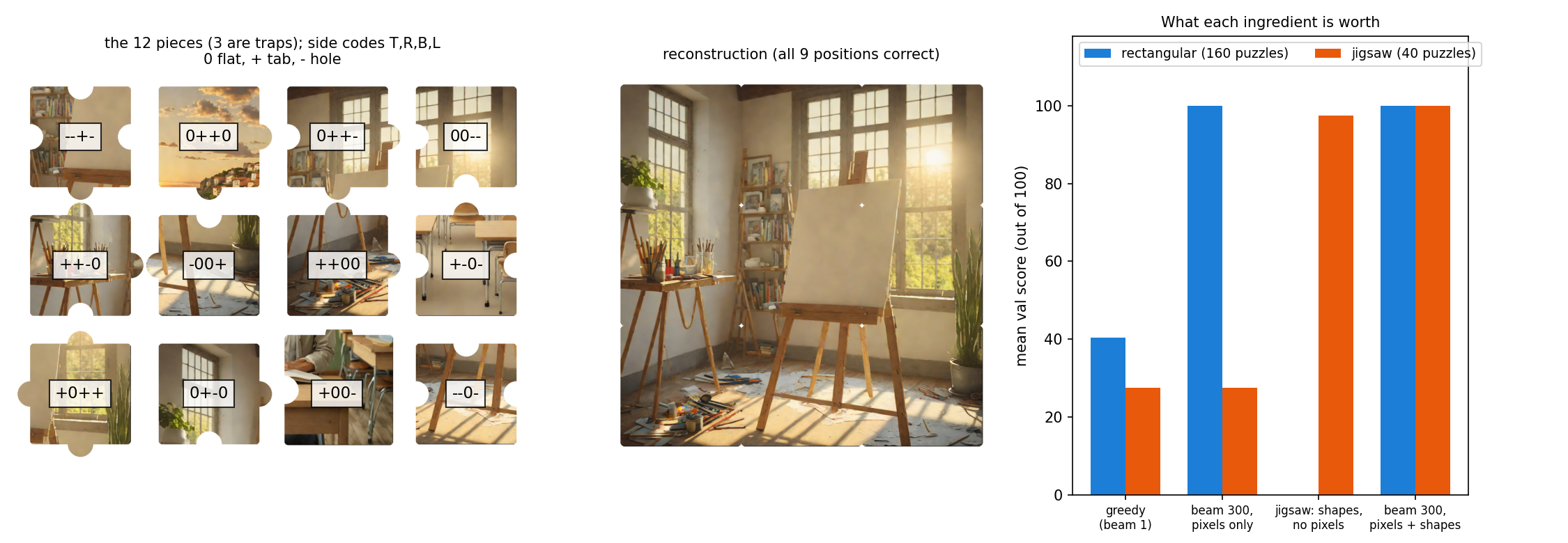
Three lessons from the table:

• Search beats greed: for square tiles, the jump from 40 to 100 comes entirely from the beam. The seam score was already good enough, the greedy search was the problem.
• For jigsaws, shapes beat pixels: shape rules alone place 97.5 % correctly, while our pixel seams alone do badly (27.6). Near a jigsaw boundary the tabs and holes leave few clean, aligned pixel pairs, and the traps are also cut as jigsaws. Combining both gives 100.
• The refinements we expected to matter, gradient extrapolation and normalisation by the second-best match, make no difference here. The images are smooth, high-resolution renders, so even raw colour differences across seams separate true neighbours well.

What to remember

• Decide jointly what a greedy pipeline decides in sequence. Choosing the pieces and placing them are one optimisation problem, and a beam search over partial solutions solves it.
• A good pairwise score plus a good search is the classic recipe for assembly problems: puzzles, document reordering, sequence reconstruction.
• Exploit hard constraints first. Flat borders and tab-hole complementarity remove most candidates for free, and hard rules are more reliable than any learned or hand-made similarity.
• Check whether a learning step is needed at all. Here the 1.7 GB training split was unnecessary: the structure of the problem (continuity across seams) was the whole model.