IOAI Training: Learn AI by solving problems

The problem in brief

Think of Shazam, but for video: you hear ten seconds of sound and must say which ten-second video clip it came from. The organisers did the heavy lifting already: every audio clip was turned into a 768-dimensional vector by WavLM (a self-supervised speech/audio model) and every video clip into a 1024-dimensional vector by V-JEPA 2 (a self-supervised video model). You get about 30,000 aligned pairs (row $i$ of the audio matrix and row $i$ of the video matrix come from the same 10 s of the same video). The test set is cut into 1,184 "samples" of 20 audios and 20 videos; inside each sample you must say, for every audio, which of the 20 videos is its partner.

The two embedding spaces were trained separately and do not even have the same dimension, so nothing can be compared directly: the whole task is to learn a bridge between two frozen encoders.

How you are scored

The metric is plain accuracy over all test audios:

\text{acc} = \frac{1}{20\,M}\sum_{m=1}^{M}\sum_{i=0}^{19} \mathbb{1}\left[\hat\pi_m(i) = \pi_m(i)\right],

where $\pi_m(i)$ is the true video of audio $i$ in sample $m$ . Random guessing gives $1/20 = 5\,\%$ . Points are piecewise linear: accuracy from 0 to 70 % maps to 0 to 20 points, and 70 to 98 % maps to 20 to 100 points, so 98 % is the full-score target (statement, "Evaluare").

The statement warns about one trap: the public leaderboard uses new clips from videos that also appear in training, while the private (final) test also contains clips from videos never seen in training. Private accuracy can therefore be lower than public accuracy. Official test labels are private, so all numbers below are on validation splits we built ourselves (see next section).

First look at the data

A few quick checks shape the whole approach:

The rows are shuffled. Consecutive training pairs are unrelated (mean cosine similarity of neighbouring video rows is $0.0008$ ), so we cannot read off which clips share a video.
Several clips come from the same video. For a random training video clip, the nearest other video clip has median cosine similarity $0.89$ (after centring), and 10 % of clips have a near-twin above $0.99$ . Clips of the same video are near-duplicates in V-JEPA space.
Audio is a weaker, noisier signal. The same nearest-neighbour test in WavLM space gives a median of $0.72$ , and the audio nearest neighbour agrees with the video nearest neighbour only 30 % of the time. A clip of street noise sounds like many other street clips.
Test samples are random draws. The highest similarity between two different videos in a test sample has the same distribution as in 20 random training clips, so there are no planted "hard negatives".

The second point matters for validation. If we hold out random pairs, the held-out clips have siblings from the same video in the training set: that imitates the public test. To imitate the private test, we need whole videos that the model never saw. Since video identities are not given, we rebuild them: connect two clips when their video cosine similarity exceeds 0.8 and take connected components as "pseudo-videos" (13,907 groups, 8,605 of them single clips). Holding out 10 % of the groups gives an unseen-video split. We evaluate on 150 random samples of 20 drawn from each split, exactly like the test.

A first baseline

The simplest bridge is linear: standardise both modalities, then fit a ridge regression $W$ that predicts the (normalised) video vector from the audio vector,

\hat W = \arg\min_W \lVert X_a W - X_v\rVert_F^2 + \lambda \lVert W\rVert_F^2 = (X_a^\top X_a + \lambda I)^{-1} X_a^\top X_v .

For each audio we then pick the video with the highest cosine similarity to $x_a \hat W$ . With $\lambda = 100$ this gives 56 % on seen videos and 48 % on unseen videos. Ten times better than chance, but only about 16 points out of 100.

A second idea exploits the near-duplicates: find the training audios closest to the test audio, average their (known) video partners into a prototype, and match the prototype. That reaches 75 % on seen videos but only 53 % on unseen ones: it is memorisation, and it is exactly the kind of method the private test is designed to punish.

The key idea

Two ideas, one about learning and one about decoding.

1. Learn a shared space with a contrastive (CLIP) loss. Regression asks the model to reproduce the whole video vector, including everything the audio cannot know (colours, camera motion). What we really need is weaker and better aligned with the metric: the true pair should score higher than the wrong pairs. So we train two small networks, an audio tower $f$ and a video tower $g$ , that map into the same 512-dimensional unit sphere, and use the symmetric InfoNCE loss on a batch of $B$ pairs:

s_{ij} = \tau^{-1}\, f(a_i)^\top g(v_j), \qquad \mathcal{L} = \frac{1}{2B}\sum_{i=1}^{B}\Big[-\log\frac{e^{s_{ii}}}{\sum_j e^{s_{ij}}} \;-\; \log\frac{e^{s_{ii}}}{\sum_j e^{s_{ji}}}\Big].

Each row is a $B$ -way classification "which video belongs to this audio?", each column the reverse question. With $B = 512$ every step is a much harder version of the 20-way test, which is precisely what we want the model to be good at. The temperature $\tau$ is learned. This is the recipe of CLIP (image and text) applied to audio and video.

2. The answer is a permutation: decode it as one. In a sample, 20 audios are matched with 20 videos and each video has exactly one audio. A row-wise argmax ignores this and happily sends three audios to the same "popular" video. The right decoder solves the assignment problem:

\hat\pi = \arg\max_{\pi \in S_{20}} \sum_{i=0}^{19} S_{i,\pi(i)},

which the Hungarian algorithm (scipy.optimize.linear_sum_assignment) solves exactly in $O(n^3)$ , instantaneous for $n = 20$ . Why does it help so much? An error under argmax usually means a wrong video looked slightly better for this audio. But that wrong video has its own true audio, which typically likes it even more. The global optimum resolves the conflict in favour of the stronger claim and pushes the weaker audio to its second choice, which is often correct. Every correct match also removes one candidate from everyone else's list.

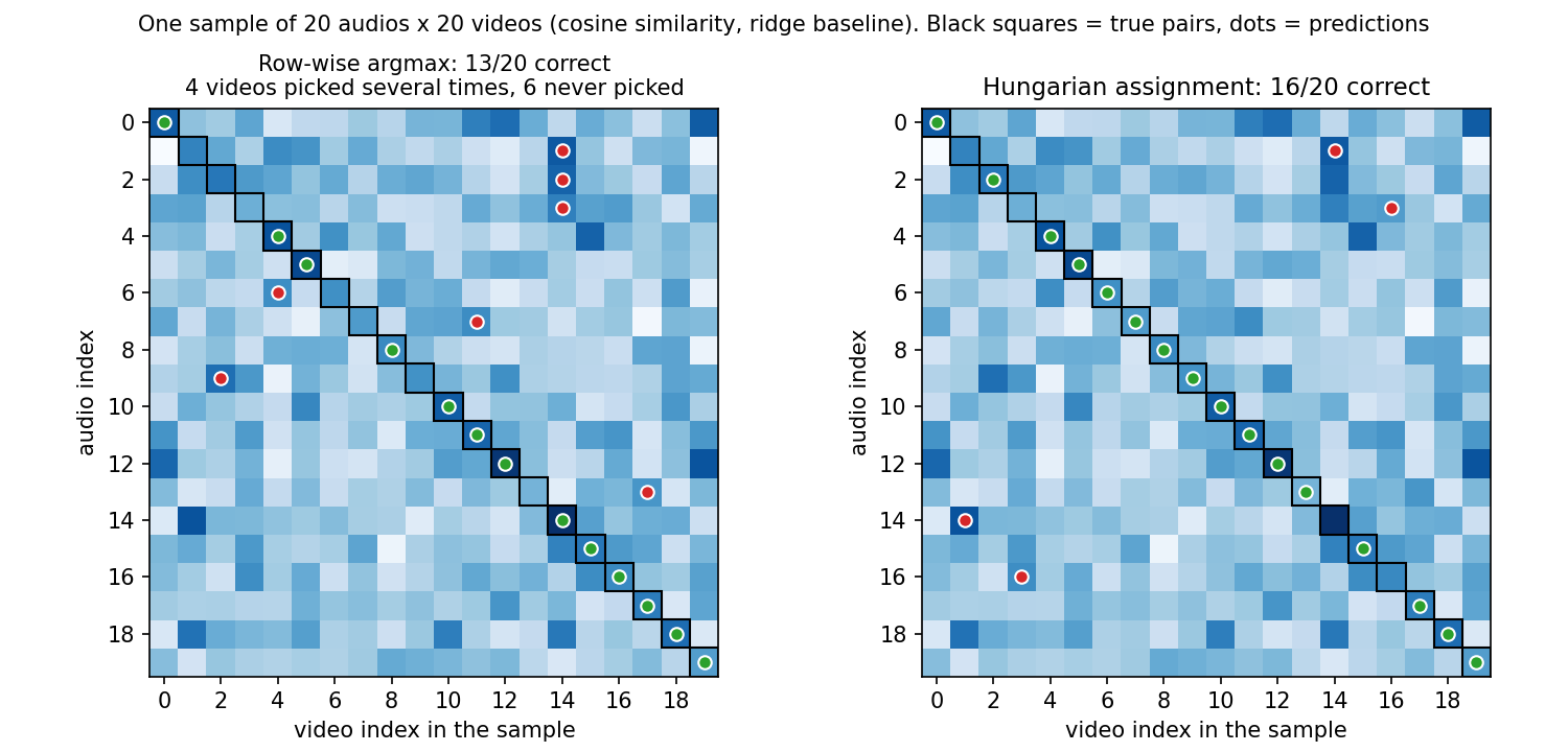
One validation sample with the ridge baseline: on the left, the row-wise argmax sends three audios to video 14 and leaves six videos unused (13/20 correct); on the right, the Hungarian assignment uses every video exactly once (16/20 correct), at the price of breaking one previously correct pair.

The figure shows a typical sample (not a cherry-picked one): the assignment fixes four errors and creates one, a net gain of three. On average, with the ridge baseline it adds +12 points on seen videos; with the contrastive model it adds +7 to +12 points, and more on the hard unseen split where argmax errors are more frequent.

The full solution

Standardise each dimension of each modality with the training mean and standard deviation (WavLM vectors have norm about 2, V-JEPA vectors about 50: without this, the towers start badly scaled).
Towers: Dropout(0.2) -> Linear(d, 1024) -> GELU -> Dropout(0.3) -> Linear(1024, 512) -> L2-normalise, one for audio ( $d=768$ ) and one for video ( $d=1024$ ). Dropout on the input is important: with only 30,000 pairs and near-duplicate clips the towers overfit quickly.
Training: AdamW (lr $10^{-3}$ , weight decay 0.05, one-cycle schedule), batch 512, 40 epochs, symmetric InfoNCE with a learnable temperature. About 2 to 4 minutes per model on 2 to 4 CPU threads.
Ensemble three towers trained with different seeds by summing their cosine-similarity matrices.
Decode each 20 x 20 matrix with the Hungarian algorithm.

The core of the training loop:

logits = log_scale.exp().clamp(max=100) * ea(Xa[b]) @ ev(Xv[b]).T   # B x B
target = torch.arange(len(b))
loss = (F.cross_entropy(logits, target) + F.cross_entropy(logits.T, target)) / 2

and the decoding:

rows, cols = linear_sum_assignment(-S)   # S = 20 x 20 similarity, maximise the total
pred[rows] = cols

Results

Accuracy on 150 random samples of 20 from each held-out split (official test labels are private).

approach	seen videos (like public test)	unseen videos (hardest part of private test)
random guess	5.0 %	5.0 %
ridge regression audio $\to$ video, argmax	56.1 %	48.0 %
ridge regression + Hungarian	68.4 %	56.0 %
nearest training audios $\to$ prototype video, argmax	74.6 %	53.1 %
contrastive towers (40 epochs), argmax	90.4 %	78.6 %
contrastive towers + Hungarian	98.1 %	91.2 %
same, hidden 2048 (+ Hungarian)	98.0 %	88.3 %
same, batch 256 (+ Hungarian)	98.1 %	88.4 %
same, 80 epochs (+ Hungarian)	98.1 %	87.7 %
contrastive + 0.3 x nearest-neighbour prototype, Hungarian	98.5 %	90.3 %
ensemble of 3 seeds + Hungarian (final)	98.7 % (argmax 91.8 %)	91.7 % (argmax 80.7 %)

(The last line comes from solution.py --val, which redraws the held-out groups with its own random seed, so it is comparable to the other lines only up to sampling noise.)

Reading the table:

The contrastive loss is the big jump (+30 points over ridge with argmax). Matching the training objective to the metric matters more than model size.
The Hungarian decoder is a free +7 to +13 points.
Bigger towers, longer training or smaller batches did not help; the differences of 2 to 3 points on the unseen split are within the noise of 150 samples (one sample is 20 answers, so the standard error is about 1 to 1.5 points).
Mixing in the memorisation trick helps a little on seen videos and hurts on unseen ones: we left it out, because the private test rewards generalisation.

On seen videos the model sits at the 98 % full-score line; on unseen videos it is around 90 %. Since the private test mixes both kinds of clips in an unknown proportion, a realistic expectation is roughly 93 to 97 % accuracy, that is about 85 to 95 points.

What to remember

When two frozen encoders must be aligned, train small projection heads with a contrastive loss that mirrors the retrieval task, rather than regressing one embedding onto the other.
Always look for structure in the output: if the answer is a permutation (or a matching, or a ranking), decode it with the right combinatorial algorithm. Hungarian matching on top of any similarity matrix is one line of SciPy.
Build the validation split the test is built like. Random splits leak near-duplicate clips of the same video; grouping clips into pseudo-videos with a similarity graph gave an honest "unseen" score and showed that memorisation tricks do not transfer.
With small, noisy data (30,000 pairs), regularisation (input dropout, weight decay) and a seed ensemble are worth more than a larger network.

"""Video Shazam (ONIA 2026, national team selection, test 1).

Given precomputed WavLM audio embeddings (768-d) and V-JEPA 2 video embeddings (1024-d),
match each of the 20 audios of a test sample to one of its 20 videos.

Pipeline
  1. Standardise each modality (per-dimension z-score, statistics from train).
  2. Train two small MLP "towers" (audio -> 512, video -> 512, L2-normalised) with the
     symmetric InfoNCE / CLIP loss: in a batch, each audio must pick its own video
     among all the others, and vice versa.
  3. Ensemble a few towers trained with different seeds (sum of cosine similarities).
  4. Inside each test sample the answer is a permutation (20 audios, 20 videos, one-to-one),
     so instead of a row-wise argmax we solve the assignment problem with the Hungarian
     algorithm on the 20x20 similarity matrix.

Run from the folder that contains data/train.pkl and data/test.pkl (the official dataset/).
Optional flag --val runs the group-held-out validation used in the write-up.
"""
import pickle
import sys
import numpy as np
import torch
import torch.nn as nn
import torch.nn.functional as F
from scipy.optimize import linear_sum_assignment

torch.set_num_threads(2)
SEEDS = [0, 1, 2]


def load(path):
    with open(path, "rb") as f:
        return pickle.load(f)


class Tower(nn.Module):
    """Input dropout -> Linear -> GELU -> dropout -> Linear -> L2 normalisation."""

    def __init__(self, d_in, hidden=1024, d_out=512, p=0.3):
        super().__init__()
        self.net = nn.Sequential(nn.Dropout(0.2), nn.Linear(d_in, hidden), nn.GELU(),
                                 nn.Dropout(p), nn.Linear(hidden, d_out))

    def forward(self, x):
        return F.normalize(self.net(x), dim=-1)


def train_towers(Xa, Xv, seed, epochs=40, bs=512, lr=1e-3, wd=0.05):
    torch.manual_seed(seed)
    ea, ev = Tower(Xa.shape[1]), Tower(Xv.shape[1])
    log_scale = nn.Parameter(torch.tensor(np.log(1 / 0.07), dtype=torch.float32))  # learnable temperature
    params = list(ea.parameters()) + list(ev.parameters()) + [log_scale]
    opt = torch.optim.AdamW(params, lr=lr, weight_decay=wd)
    steps = epochs * (len(Xa) // bs)
    sched = torch.optim.lr_scheduler.OneCycleLR(opt, lr, total_steps=steps)
    for _ in range(epochs):
        ea.train(); ev.train()
        perm = torch.randperm(len(Xa))
        for i in range(len(Xa) // bs):
            b = perm[i * bs:(i + 1) * bs]
            logits = log_scale.exp().clamp(max=100) * ea(Xa[b]) @ ev(Xv[b]).T
            target = torch.arange(len(b))
            loss = (F.cross_entropy(logits, target) + F.cross_entropy(logits.T, target)) / 2
            opt.zero_grad(); loss.backward(); opt.step(); sched.step()
    ea.eval(); ev.eval()
    return ea, ev


class Matcher:
    def __init__(self, A, V):
        self.mA, self.sA = A.mean(0), A.std(0) + 1e-6
        self.mV, self.sV = V.mean(0), V.std(0) + 1e-6
        Xa = torch.tensor((A - self.mA) / self.sA, dtype=torch.float32)
        Xv = torch.tensor((V - self.mV) / self.sV, dtype=torch.float32)
        self.towers = [train_towers(Xa, Xv, s) for s in SEEDS]

    @torch.no_grad()
    def similarity(self, a, v):
        a = torch.tensor((a - self.mA) / self.sA, dtype=torch.float32)
        v = torch.tensor((v - self.mV) / self.sV, dtype=torch.float32)
        return sum((ea(a) @ ev(v).T).numpy() for ea, ev in self.towers)

    def predict(self, a, v):
        S = self.similarity(a, v)
        rows, cols = linear_sum_assignment(-S)  # maximise total similarity, one video per audio
        pred = np.empty(len(a), dtype=int)
        pred[rows] = cols
        return pred


def validate(A, V):
    """Two held-out sets: random pairs (videos seen in training) and whole pseudo-videos never seen.
    Pseudo-videos = connected components of the graph 'video cosine similarity > 0.8'."""
    from scipy.sparse import csr_matrix
    from scipy.sparse.csgraph import connected_components
    rng = np.random.default_rng(0)
    Vn = V - V.mean(0); Vn /= np.linalg.norm(Vn, axis=1, keepdims=True)
    r, c = [], []
    for s in range(0, len(V), 2000):
        rr, cc = np.nonzero(Vn[s:s + 2000] @ Vn.T > 0.8); r += list(rr + s); c += list(cc)
    _, group = connected_components(csr_matrix((np.ones(len(r)), (r, c)), shape=(len(V),) * 2))
    held = set(rng.choice(np.unique(group), int(0.1 * group.max()), replace=False))
    unseen = np.array([g in held for g in group])
    seen = rng.permutation(np.nonzero(~unseen)[0])
    val_seen, train_idx, val_unseen = seen[:3000], seen[3000:], np.nonzero(unseen)[0]
    m = Matcher(A[train_idx], V[train_idx])
    for name, ix in [("seen videos", val_seen), ("unseen videos", val_unseen)]:
        acc_arg, acc_hun = [], []
        for _ in range(150):
            s = rng.choice(ix, 20, replace=False)
            S = m.similarity(A[s], V[s])
            acc_arg.append(np.mean(S.argmax(1) == np.arange(20)))
            acc_hun.append(np.mean(m.predict(A[s], V[s]) == np.arange(20)))
        print(f"{name:14s} argmax {np.mean(acc_arg):.3f}   hungarian {np.mean(acc_hun):.3f}")


if __name__ == "__main__":
    train = load("./data/train.pkl")
    A, V = train["audio_embeddings"], train["video_embeddings"]
    if "--val" in sys.argv:
        validate(A, V)
        sys.exit()
    matcher = Matcher(A, V)  # final model: all 29,994 training pairs
    test = load("./data/test.pkl")
    with open("./submission.csv", "w") as f:
        f.write("subtaskID,sample_id," + ",".join(str(i) for i in range(20)))
        for sample in test:
            pred = matcher.predict(sample["audio_embeddings"], sample["video_embeddings"])
            f.write(f"\n1,{sample['sample_id']}," + ",".join(str(p) for p in pred))
    print("wrote submission.csv with", len(test), "samples")