IOAI Training: Learn AI by solving problems

The problem in brief

You receive infrared satellite images of typhoons over the Western Pacific, each centred on the storm, and must estimate the storm's central pressure in hectopascals. The lower the pressure, the stronger the typhoon: about 1 000 hPa for a tropical storm, around 900 hPa for a super typhoon. Training data: 5 000 labelled images from 2010 to 2019 (106 storms, from three Japanese geostationary satellites). Test data: 1 000 images from the 2020 season, whose labels are kept by the organisers. The images come from the public Digital Typhoon dataset (Kitamoto Lab, NII), so the 2020 answers exist online: looking them up would be cheating, and we did not.

Because the test labels are private, every score below is a validation score: we train on 2010 to 2017 and validate on the 1 020 images of 2018 and 2019.

How you are scored

The submission is a CSV with one predicted pressure per test image, scored by root mean squared error:

\text{RMSE} = \sqrt{\frac{1}{N}\sum_{i=1}^{N} \left(\hat p_i - p_i\right)^2}\quad\text{(hPa, lower is better).}

RMSE squares the errors, so a few large misses on intense storms weigh much more than many small errors on weak ones. No threshold or leaderboard has been published for this task.

First look at the data

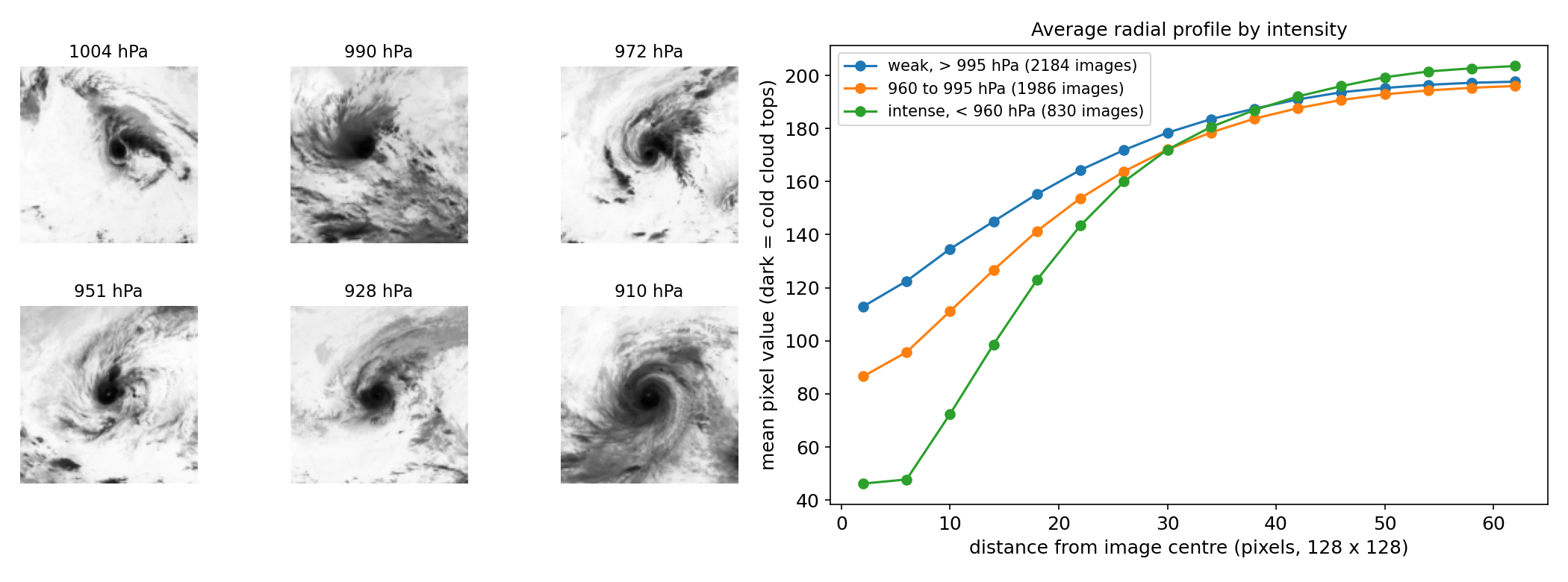
Six training images at different pressures, and the average radial brightness profile

What the image shows. In these infrared images, dark means cold, and cold means high cloud tops, i.e. deep convection. An intense typhoon has a compact, very cold, symmetric ring of convection around a well-defined eye; a weak storm is a ragged, warmer cloud mass. The right panel shows it on average: the strongest storms (green) are much darker within 20 pixels of the centre, and the profile is steeper.
Rotation does not matter. A storm photographed rotated by 90 degrees, or mirrored, has the same intensity. This is a symmetry we can exploit.
Images are not independent. The data contains many consecutive hourly images of the same storm (about 45 per storm on average), which look almost the same and have almost the same label. A random train/validation split would put near-duplicates on both sides and give an absurdly optimistic score. The official test is a different year, so we split by year: 2018 and 2019 for validation.
Imbalance in intensity. Half the images are above 992 hPa; only 830 are below 960 hPa. The rare intense storms carry most of the RMSE.

A first baseline

Predicting the training mean for every image gives an RMSE of 25.9 hPa. A physically inspired baseline turns each image into a radial profile: for 16 rings of 4 pixels around the centre, the mean, standard deviation and 10th and 90th percentiles of brightness, plus the share of very bright and dark pixels (67 numbers). This is close to what meteorologists did for decades with the Dvorak technique, which reads intensity from cloud patterns around the centre. Ridge regression on these features reaches 16.4 hPa, and gradient-boosted trees 14.5 hPa. Good, but the left panel of the results figure shows the limit: the profile cannot see the structure (a clear eye, spiral bands, symmetry), so intense storms are often underestimated.

The key idea

Let a CNN learn the cloud patterns, and teach it the symmetry of the problem through augmentation.

A convolutional network sees exactly what the radial profile misses: the shape of the eye, how closed the ring of convection is, the curvature of the bands. But with only about 4 000 training images from 85 storms, a CNN can memorise individual storms. Two tricks make it generalise:

The 8 symmetries of the square. At every training step the batch is rotated by 0, 90, 180 or 270 degrees and possibly mirrored. Intensity is invariant to these transformations, so we get 8 versions of every image for free, and the network cannot rely on the orientation of a particular storm's bands. At prediction time we average the 8 predictions (test-time augmentation). One might object that typhoons in the Northern Hemisphere always spin counter-clockwise, which a mirror reverses; in practice the network gains more from the extra data than it loses from that detail.
Small random shifts (up to 6 pixels): the storm centre in the images is not perfectly aligned, and the prediction should not depend on it.

Without augmentation the same network reaches 10.4 hPa; with it, 9.6 hPa. The loss is smooth L1 (Huber) on the standardised pressure, which behaves like MSE for small errors but is less dominated by a few badly labelled or atypical images during training.

The full solution

Resize the 512 x 512 PNGs to 128 x 128 grey-scale arrays and scale pixels to $[-0.5, 0.5]$ .
Network: five blocks of two 3 x 3 convolutions with batch normalisation and ReLU, each followed by 2 x 2 max-pooling (32 to 256 channels, 128 to 4 pixels), global average pooling, dropout 0.3, and one linear output.
Train 30 epochs with AdamW, batch 64, one-cycle learning rate up to $2 \times 10^{-3}$ , smooth L1 loss on $(p - \mu)/\sigma$ , with random D4 symmetry and shifts. About 5 minutes on an Apple GPU.
Predict with the average over the 8 symmetries; for the submission, train on all 5 000 images with 3 different seeds and average them.

def d4(x, k):                      # k-th symmetry of the square
    x = torch.rot90(x, k % 4, (2, 3))
    return x.flip(3) if k >= 4 else x
pred = torch.stack([net(d4(xb, k)) for k in range(8)]).mean(0)

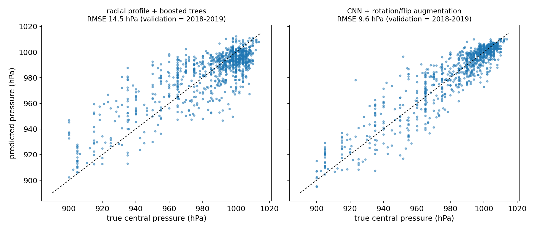
Predicted against true pressure on the 2018-2019 validation images

Where are the errors? Split by intensity, the CNN's validation RMSE is 5.8 hPa for weak storms (above 990 hPa) but 14 to 16 hPa below 970 hPa, and the most intense storms (below 940 hPa) are predicted 7 hPa too weak on average. This is regression to the mean: the rare extreme cases are pulled towards the bulk of the data. It is also physically hard, since storms of very different pressures can look similar at a given moment (a storm may be intensifying or weakening). Blending 20 % of the boosted-tree prediction into the CNN improves validation only marginally (9.46), so we kept the single, simpler model.

Results

Validation = all 1 020 images from 2018 and 2019, models trained on 2010 to 2017 (the official 2020 test labels are private).

approach	validation RMSE (hPa)
predict the training mean	25.9
radial profile (67 features) + ridge regression	16.4
radial profile + gradient-boosted trees	14.5
CNN, no augmentation	10.4
CNN + D4 symmetries + shifts + 8-fold TTA (final)	9.6
final CNN blended with 20 % boosted trees	9.5

The submission averages 3 seeds of the final CNN trained on all 10 years.

What to remember

Split like the test. Consecutive images of the same storm are near-duplicates; validating on whole years (here 2018-2019, like the 2020 test) is the only honest estimate.
Encode known invariances as augmentation. Intensity does not depend on orientation, so rotations and reflections multiply the data by 8 and cut the error by about 8 % here; averaging the 8 views at test time adds a little more.
Start from physics, then let the model see more. A radial profile captures the main signal (cold, compact centre) and halves the naive error; the CNN wins by reading structure the profile cannot express.
RMSE lives in the tails. The rare intense storms dominate the error; check errors per intensity range, not just the global number.
Public data can contain the answers. The test images come from a public dataset; using its labels would be cheating, so build the model as if they did not exist.

Note on the code. The full solution.py below was assembled from scripts that did run, but it was not re-run end to end after assembly.

"""Typhoon Intensity Estimation (IOAI Philippines 2026 finals, practical 1).

Predict the central pressure (hPa) of a typhoon from one infrared satellite image; metric RMSE.
Train = 2010-2019 (5000 images), test = 2020 (1000 images, labels private).
Validation mimics the test: train on 2010-2017, validate on 2018-2019 (never a random split:
consecutive hourly images of the same storm are almost identical).

Model: a small CNN on 128x128 images, trained with the 8 symmetries of the square (rotations and
reflections) and small shifts as augmentation, smooth-L1 loss on the standardised pressure,
test-time averaging over the 8 symmetries, and an average of 3 seeds for the final submission.
Usage: python solution.py val          -> validation RMSE (2018-2019)
       python solution.py full         -> submission.csv for the 2020 test images
Data: img/train.csv, img/test.csv, img/train_images/*.png, img/test_images/*.png (512x512 grey PNG)
"""
import os, sys, numpy as np, pandas as pd, torch, torch.nn as nn, torch.nn.functional as F
from PIL import Image
torch.set_num_threads(2)
DEV = "mps" if torch.backends.mps.is_available() else ("cuda" if torch.cuda.is_available() else "cpu")
MODE = sys.argv[1] if len(sys.argv) > 1 else "val"
EPOCHS, BS = 30, 64


def load(folder, names, cache):
    if os.path.exists(cache): return np.load(cache)
    X = np.stack([np.asarray(Image.open(f"{folder}/{n}").convert("L").resize((128, 128), Image.BILINEAR))
                  for n in names]).astype(np.uint8)
    np.save(cache, X); return X

tr, te = pd.read_csv("img/train.csv"), pd.read_csv("img/test.csv")
X = load("img/train_images", tr.filename, "X_train128.npy"); XE = load("img/test_images", te.filename, "X_test128.npy")
y = tr.label.values.astype(np.float32)
va = (tr.filename.str[:4].astype(int) >= 2018).values.copy()    # filename starts with YYYYMMDDHH
if MODE == "full": va[:] = False


def block(i, o):
    return nn.Sequential(nn.Conv2d(i, o, 3, padding=1, bias=False), nn.BatchNorm2d(o), nn.ReLU(),
                         nn.Conv2d(o, o, 3, padding=1, bias=False), nn.BatchNorm2d(o), nn.ReLU(), nn.MaxPool2d(2))

def make_net():     # 128 -> 64 -> 32 -> 16 -> 8 -> 4, then global average pooling
    return nn.Sequential(block(1, 32), block(32, 64), block(64, 128), block(128, 256), block(256, 256),
                         nn.AdaptiveAvgPool2d(1), nn.Flatten(), nn.Dropout(0.3), nn.Linear(256, 1)).to(DEV)

to_t = lambda a: (torch.tensor(a, dtype=torch.float32) / 255. - 0.5).unsqueeze(1)

def d4(x, k):
    """The k-th of the 8 symmetries of the square: a storm seen rotated or mirrored keeps its intensity."""
    x = torch.rot90(x, k % 4, (2, 3)); return x.flip(3) if k >= 4 else x


def train_one(seed):
    torch.manual_seed(seed); np.random.seed(seed)
    mu, sd = y[~va].mean(), y[~va].std()
    net = make_net(); Xt, Yt = to_t(X[~va]), torch.tensor((y[~va] - mu) / sd)
    opt = torch.optim.AdamW(net.parameters(), 1e-3, weight_decay=1e-4)
    sched = torch.optim.lr_scheduler.OneCycleLR(opt, 2e-3, total_steps=EPOCHS * (len(Yt) // BS))
    for ep in range(EPOCHS):
        net.train(); perm = torch.randperm(len(Yt))
        for i in range(0, len(Yt) - BS + 1, BS):
            b = perm[i:i + BS]; xb = d4(Xt[b].to(DEV), np.random.randint(8))
            dx, dy = np.random.randint(-6, 7, 2)                    # the eye is not exactly centred
            xb = torch.roll(xb, (int(dx), int(dy)), (2, 3))
            loss = F.smooth_l1_loss(net(xb).squeeze(1), Yt[b].to(DEV), beta=0.5)
            opt.zero_grad(); loss.backward(); opt.step(); sched.step()

    @torch.no_grad()
    def predict(A):
        net.eval(); out = []
        for i in range(0, len(A), 128):
            xb = to_t(A[i:i + 128]).to(DEV)
            out.append(torch.stack([net(d4(xb, k)).squeeze(1) for k in range(8)]).mean(0).cpu())
        return torch.cat(out).numpy() * sd + mu
    return predict


if MODE == "val":
    p = train_one(0)(X[va])
    print(f"validation RMSE (2018-2019): {np.sqrt(((p - y[va]) ** 2).mean()):.2f} hPa "
          f"(predicting the mean: {np.sqrt(((y[~va].mean() - y[va]) ** 2).mean()):.2f})")
else:
    preds = np.mean([train_one(s)(XE) for s in range(3)], axis=0)
    pd.DataFrame({"id": te.filename, "label": preds}).to_csv("submission.csv", index=False)
    print("submission.csv written", preds.min(), preds.max())