IOAI Training: Learn AI by solving problems

The problem in brief

You receive 500 infrared satellite images of Hurricane Beryl (June-July 2024), each labelled with the storm's maximum sustained wind in knots, and 500 unlabelled images of Hurricane Milton (October 2024). You must predict Milton's wind speed from the pixels alone: an automated version of the Dvorak technique that forecasters use to read intensity from cloud patterns. Looking up Milton's real intensities is explicitly forbidden, and so is exploiting the timestamps. What makes the task hard is not the images but the split: training on one storm and testing on another storm, in a different ocean basin, that becomes stronger (155 kt) than anything in the training set (145 kt).

How you are scored

Root mean squared error over the 500 Milton images, lower is better:

\text{RMSE} = \sqrt{\frac{1}{n}\sum_{i=1}^{n} (y_i - \hat y_i)^2}.

The organisers publish no threshold, and the test labels are private. Because Milton is a historical storm, its official NHC best track is public; we used it only after freezing our models, to estimate how they would score, never to fit or tune anything. Since we do not know exactly how the organisers built Milton's labels, we report two proxies: the daily maximum of the best track (this rule reproduces Beryl's training labels, see below) and the best track interpolated in time. Treat them as approximate test scores.

First look at the data

The images. These are colour-enhanced IR pictures (640 x 480, GOES-16 band 13) in which colour encodes cloud-top temperature: grey and white for warm, low clouds, then blue, green, red and finally yellow for the coldest, highest tops, which mark the most vigorous convection. A banner at the bottom carries the colour bar and also the date and time: a model could read the date from it, so we crop it away.

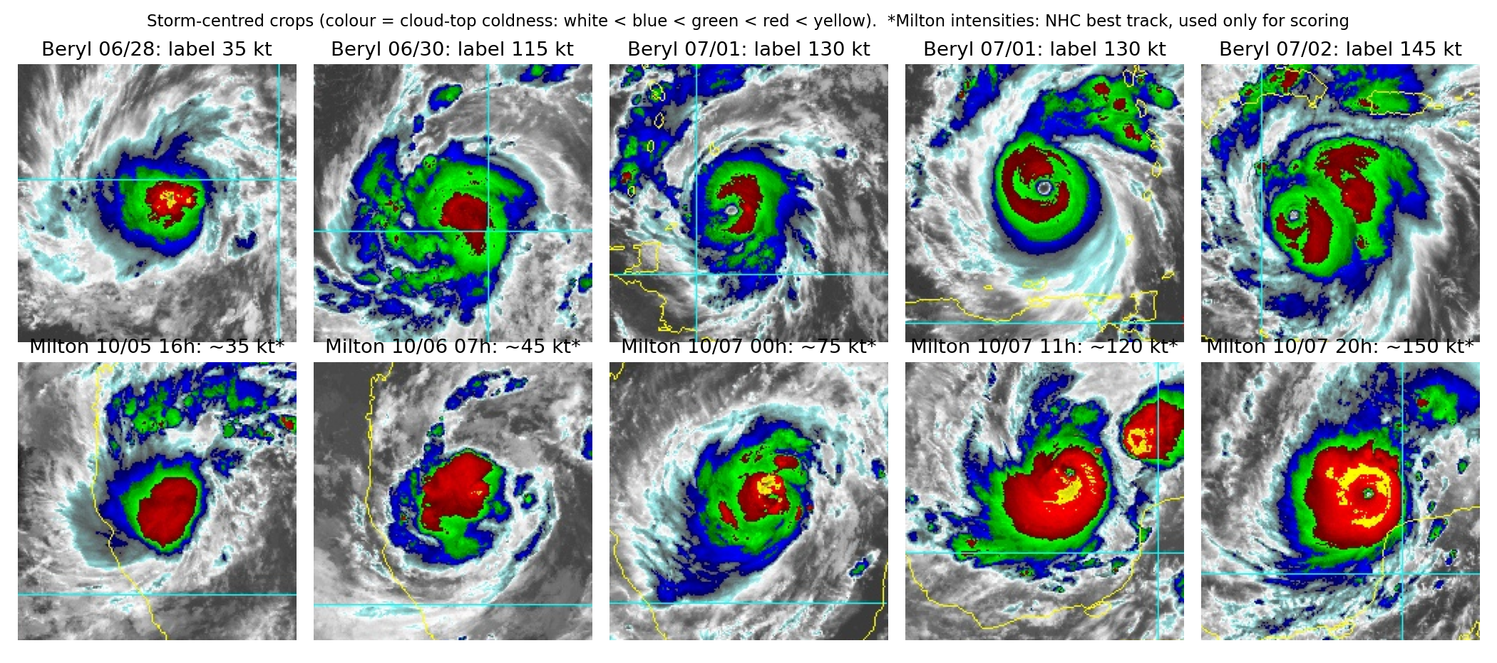
Storm-centred crops of Beryl (top) and Milton (bottom). Beryl's strong stages show a clear eye inside a closed green and red ring. Milton is covered by a huge red and yellow cloud shield already at tropical-storm strength, and its eye at 150 kt is only a few pixels wide.

The labels are coarse. Beryl's 500 labels take only five values, one per calendar day: 35, 65, 115, 130 and 145 kt. Comparing with the public best track shows they are the daily maximum: for example, every image of 30 June is labelled 115 kt, although Beryl was at 70 kt at midnight and only reached 115 kt at 18 UTC. So a 01:30 image of a 70 kt storm is labelled 115 kt. Three consequences:

there are really only five independent training targets, not 500;
consecutive frames (10 minutes apart) are near-duplicates, so a random train/validation split leaks and gives absurdly optimistic scores;
even a perfect "physical" model cannot reach a low RMSE against such labels.

The test storm looks different. Milton grew in the Gulf of Mexico, where the convection was much colder: on 5 October, at only 35 kt, it already shows a red cloud mass larger than Beryl's at 130 kt. And at peak intensity its eye is a pinhole of 2 to 3 pixels.

A first baseline

A constant prediction is the reference. Predicting the training mean (109 kt) everywhere gives a proxy RMSE around 50 kt; the sample submission's constant 75 kt gives 39 to 54 kt depending on the proxy. To validate on Beryl honestly we use leave-one-day-out cross-validation: train on four days, predict the fifth. A constant gets 41.6 kt this way.

The key idea

The decisive idea is a validation question, not a model: what does my validation measure? Leave-one-day-out on Beryl measures generalisation to another day of the same storm. The test is generalisation to another storm. These are different things, and on this task they disagree.

We first built features in the obvious way. The colour bar in each image gives a lookup from colour to a "coldness" value between 0 (warm) and 1 (coldest), then we locate the storm centre (the densest patch of blue-or-colder pixels) and measure, inside discs of radius 20, 40, 80 and 140 pixels, the fraction of pixels colder than each colour level. That is 20 "cloud-area" numbers per image. A ridge regression on them gets the best leave-one-day-out score of everything we tried, 18.9 kt, much better than a pretrained ResNet-18 embedding (23.9 kt).

On Milton it collapses (proxy RMSE 44 to 54 kt): it predicts about 100 kt for the 35 kt tropical storm, because Milton's cold cloud shield is huge from the start. The model has learned "more cold cloud means stronger" from one storm, which is a correlation of Beryl's life cycle, not a law of physics. With five effective training targets and 20 features, the ridge can essentially memorise which day an image comes from.

The physics says something more specific. The Dvorak technique estimates intensity mainly from the eye and the ring of cold cloud around it: a strong hurricane has a warm, well-defined eye enclosed by a complete ring of very cold tops; a weak storm has a cold blob without a clear eye, however large. So we built only four features that follow that logic:

eye_score: the largest contrast between a warm pixel and the coldest-closed ring of radius 5 to 12 pixels around it;
eyewall_q10: the 10th percentile of coldness on that ring, i.e. how cold the weakest point of the eyewall is (a broken ring has a warm gap, so its 10th percentile is low);
eye_c: how warm the eye itself is;
cdo_mean: mean coldness of the central dense overcast within 40 pixels.

Using a percentile of the ring rather than its mean is the important detail: it rewards a closed, symmetric eyewall, the visual signature that separates a 150 kt "buzzsaw" from a lopsided burst of convection.

This 4-feature model is worse in leave-one-day-out (34.8 kt) but clearly better on Milton (proxy RMSE 30.5 to 38.8 kt): it correctly keeps the early tropical storm near 60 to 75 kt and rises during the explosive intensification.

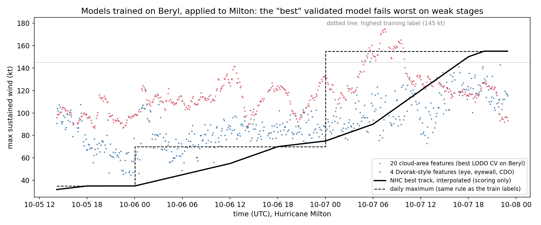
Predictions over Milton's life cycle. The 20-feature cloud-area model predicts around 100 kt from the start and spikes to 175 kt; the 4-feature Dvorak-style model starts near 60 to 90 kt and climbs to about 120 kt at the end. The black curves show the best track rising from 35 to 155 kt.

Honesty note: we chose the 4-feature model after seeing the proxy scores of the first one, so its proxy score is somewhat optimistic. A choice we could have defended in advance is the principle behind it: with only five independent labels and a known distribution shift, prefer few, physically motivated features over many correlated ones, even at the cost of in-domain validation.

The full solution

Coldness map. Read the colour bar from the banner (rows 456 to 467), build a lookup table from RGB to the position of the nearest colour-bar entry, and drop the banner rows.
Centre. Smooth the mask "colder than blue" with a Gaussian of 15 pixels and take its maximum.
Eye and eyewall. On a 141 x 141 window around the centre, compute a 10th-percentile filter over an annulus (radius 5 to 12 px) and pick the pixel that maximises "ring coldness minus pixel coldness":

ring = percentile_filter(w, 10, footprint=ANNULUS)   # weakest point of a ring
score = ring - w                                      # closed cold ring around a warm spot
iy, ix = np.unravel_index(score.argmax(), score.shape)
feats = dict(eye_score=score[iy, ix], eyewall_q10=ring[iy, ix],
             eye_c=w[iy, ix], cdo_mean=w[30:111, 30:111].mean())

Model. Standardise the four features and fit a ridge regression (alpha by internal CV). A linear model can extrapolate a little beyond 145 kt, which trees cannot do at all.
Validation. Leave-one-day-out on Beryl; then, once frozen, proxy scoring against Milton's best track.

Results

approach	leave-one-day-out RMSE (Beryl)	proxy test RMSE, daily max	proxy test RMSE, interpolated
constant 75 kt (sample submission)	n/a	53.5	39.3
constant training mean (109 kt)	41.6	49.3	50.4
ResNet-18 ImageNet features + ridge	23.9	48.2	50.9
20 cloud-area features, extra trees	22.5	not run	not run
20 cloud-area features + ridge	18.9	44.0	53.6
same, plus temporal median filter over 13 frames	n/a	43.7	53.3
cloud areas + Dvorak features, ridge	18.2	43.4	50.6
4 Dvorak-style features + ridge (final)	34.8	38.8	30.5

All rows are in knots. The ranking by validation on Beryl is almost exactly the reverse of the ranking on Milton. Even the final model is far from good: it never predicts above about 145 kt, and Milton's pinhole eye is too small for our 2-pixel smoothing, so the peak is underestimated by 30 kt or more. Possible next steps, not tried here: detecting the eye at full resolution without smoothing, adding the radius of the coldest closed ring as Dvorak does, and training on more storms (which the rules forbid here).

What to remember

Count your independent labels. 500 images with 5 distinct, day-level labels is a 5-example problem; that dictates both the validation scheme and how many features you can afford.
Group your validation by the unit of correlation (here the day), never split near-duplicate frames at random.
Validation should mimic the test shift. In-storm validation rewarded the model that generalised worst to a new storm. When the test domain differs, simple features grounded in the physics travel better than many correlated ones.
Read the labels against a reference. Recognising "daily maximum" labels explains much of the error that no model can remove.
Remove leaks on purpose: crop the banner that prints the date, and never let public test answers touch training or tuning.

"""IOAI Philippines 2026 National Finals, Practical 2: The Eye of the Storm.
Train on Hurricane Beryl IR images, predict max sustained wind (kt) for Hurricane Milton.
Data: github.com/ioaiph/2026, folder "Finals/Practical 2" (sparse checkout into work/repo).
Pipeline: colour-enhanced IR -> cloud-top "coldness" map via the image's own colour bar
-> storm centre -> Dvorak-style features (eye, eyewall, central dense overcast) -> ridge.
"""
import numpy as np, pandas as pd
from PIL import Image
from scipy.ndimage import gaussian_filter, percentile_filter
from sklearn.linear_model import RidgeCV
from sklearn.pipeline import make_pipeline
from sklearn.preprocessing import StandardScaler

B = "work/repo/Finals/Practical 2/Data/"
IMG = B + "Atlantic_Finals_Dataset/"
tr, te = pd.read_csv(B + "train.csv"), pd.read_csv(B + "test.csv")

# 1. Colour -> coldness. Each McIDAS image carries its colour bar in the bottom banner
#    (rows 456-467, columns 110-590, warm on the left, cold on the right). Every pixel is
#    mapped to the position (0 = warm, 1 = cold) of its nearest colour-bar entry.
ref = np.array(Image.open(IMG + "Beryl/" + tr.Filename[0])).astype(float)
pal = ref[456:468, 110:590].mean(0)
g = np.arange(0, 256, 4) + 2
grid = np.stack(np.meshgrid(g, g, g, indexing="ij"), -1).reshape(-1, 3)
near = np.concatenate([np.argmin(((grid[i:i + 20000, None] - pal[None]) ** 2).sum(-1), 1)
                       for i in range(0, len(grid), 20000)])
LUT = np.linspace(0, 1, len(pal))[near].reshape(64, 64, 64).astype(np.float32)

def coldness(path):
    a = np.array(Image.open(path))[:455] // 4      # drop the banner (it also holds the date!)
    return LUT[a[..., 0], a[..., 1], a[..., 2]]

BLUE = 0.79                                         # colour-bar position where blue starts
ann_y, ann_x = np.mgrid[-15:16, -15:16]
ANNULUS = (np.hypot(ann_y, ann_x) >= 5) & (np.hypot(ann_y, ann_x) <= 12)

def features(c):
    # storm centre = densest patch of deep convection (blue or colder), away from the borders
    deep = gaussian_filter((c > BLUE).astype(np.float32), 15)
    deep[:60] = deep[-60:] = 0; deep[:, :80] = deep[:, -80:] = 0
    cy, cx = np.unravel_index(deep.argmax(), deep.shape)
    s = gaussian_filter(c, 1)
    w = np.pad(s, 80, mode="edge")[cy + 10: cy + 151, cx + 10: cx + 151]   # 141x141 window
    # eye search: a warm pixel surrounded by a CLOSED cold ring. The 10th percentile of the
    # ring of radius 5-12 px is the coldness of its weakest point (Dvorak's "surrounding ring").
    ring = percentile_filter(w, 10, footprint=ANNULUS)
    score = ring - w
    score[:15] = score[-15:] = -1; score[:, :15] = score[:, -15:] = -1
    iy, ix = np.unravel_index(score.argmax(), score.shape)
    return {"eye_score": score[iy, ix], "eyewall_q10": ring[iy, ix], "eye_c": w[iy, ix],
            "cdo_mean": w[30:111, 30:111].mean()}

F = pd.DataFrame([features(coldness(IMG + "Beryl/" + f)) for f in tr.Filename])
FT = pd.DataFrame([features(coldness(IMG + "Milton/" + f)) for f in te.Filename])
y, day = tr.WindSpeed.values, tr.Filename.str[18:26].values

# 2. Validation: all images of one day share one label, and consecutive frames are
#    near-duplicates, so a random split leaks. Leave-one-day-out (5 folds) instead.
model = lambda: make_pipeline(StandardScaler(), RidgeCV(alphas=np.logspace(-2, 3, 20)))
pred = np.zeros(len(y))
for d in np.unique(day):
    m = day == d
    pred[m] = model().fit(F[~m], y[~m]).predict(F[m])
print("leave-one-day-out RMSE: %.1f kt" % np.sqrt(((pred - y) ** 2).mean()))

# 3. Fit on all of Beryl, predict Milton
final = model().fit(F, y)
out = final.predict(FT)
pd.DataFrame({"Filename": te.Filename, "WindSpeed": out.round(1)}).to_csv("work/submission.csv", index=False)
print(pd.Series(out).groupby(te.Filename.str[18:26]).mean().round(1))

# 4. SCORING ONLY, after the model is frozen: NHC best track of Milton (public HURDAT2),
#    never used for training or for any choice inside this script.
bt = pd.Series([30, 35, 35, 45, 55, 70, 75, 90, 120, 150, 155], index=pd.to_datetime([
    "2024-10-05 12:00", "2024-10-05 18:00", "2024-10-06 00:00", "2024-10-06 06:00", "2024-10-06 12:00",
    "2024-10-06 18:00", "2024-10-07 00:00", "2024-10-07 06:00", "2024-10-07 12:00", "2024-10-07 18:00",
    "2024-10-07 20:00"]))
t = pd.to_datetime(te.Filename.str[18:30], format="%Y%m%d%H%M")
y_interp = np.interp(t.astype("int64"), bt.index.astype("int64"), bt.values)
y_daymax = te.Filename.str[18:26].map({"20241005": 35, "20241006": 70, "20241007": 155}).values
for name, yt in [("daily-max proxy", y_daymax), ("interpolated proxy", y_interp)]:
    print("%s RMSE: %.1f kt" % (name, np.sqrt(((out - yt) ** 2).mean())))