IOAI Training: Learn AI by solving problems

The problem in brief

Each Andean textile is known only through a $32\times32$ grid of real numbers, a fragment taken from one of its corners. You have to predict its value. The twist is the factory rule: the model must be scikit-learn's LinearRegression with default settings, on at most 100 features, and the whole pipeline (features, training, inference) must run within 60 seconds on a CPU. Supervised models may not be used to build features. Unsupervised methods are allowed. The whole game is therefore feature engineering. You get 40 000 training fragments and 20 000 labelled validation fragments ("live test"), plus 40 000 final-test fragments without labels.

The organisers' final-test values are not published, so every score below is on the official validation set, which we never trained on.

How you are scored

The metric is the root mean square error:

\text{RMSE} = \sqrt{\frac{1}{N}\sum_{i=1}^{N} (\hat y_i - y_i)^2 } .

The values are around 1662, with a standard deviation of 97.5, so always predicting the mean gives RMSE 97.5. The organisers publish team points per question on the OPEIA 2025 results page, but no RMSE threshold, so there is no numerical target to compare with.

First look at the data

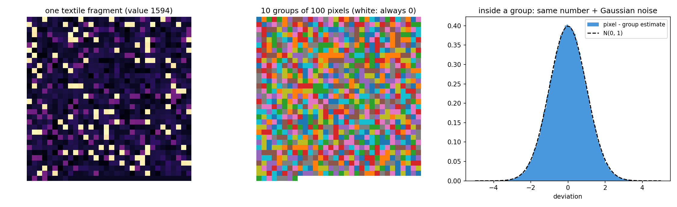
The fragments do not look like textiles at all. Most entries are small numbers (around 0 to 8), some sit near 20, others near 70. A few images contain enormous spikes, as large as $\pm 4600$ . Plotting several fragments side by side shows something more striking: the bright pixels are at the same positions in every image. The layout is fixed, so the pixels play the role of columns in a disguised table.

To find the table's columns without using the labels, compute the correlation between every pair of pixels across 20 000 images (after clipping the spikes) and link pixels whose correlation exceeds 0.3. The connected components are remarkably clean:

10 groups of exactly 100 pixels each, scattered over the grid;
the last 24 pixels of the bottom row are always exactly 0.

Inside a group, all pixels have the same median, and each one deviates from the group value by noise that is exactly $\mathcal N(0,1)$ : every pixel's noise standard deviation lies between 0.98 and 1.02, and the deviations are uncorrelated between groups. About 1 % of images also carry the huge spikes.

So the generator is: draw 10 hidden numbers $z_0,\dots,z_9$ (eight are Gaussian; $z_2$ and $z_7$ have skewness 2 and kurtosis 6, the signature of exponential distributions), copy each into 100 pixels, add unit Gaussian noise, sprinkle a few spikes, and shuffle the positions.

A fragment, its hidden group structure, and the noise inside a group

A first baseline

The organisers' dummy extractor keeps the first 100 raw pixels. It scores RMSE 181, almost twice as bad as predicting the mean. It sees only a noisy, partial view of a few groups, and the spikes wreck the least-squares fit: a single pixel at 4000 creates an enormous residual.

The key idea

Measure each hidden number as precisely as possible, robustly to outliers, and the linear model does the rest.

If $\varepsilon_k \sim \mathcal N(0,1)$ independently, the average of 100 copies $z + \varepsilon_k$ has noise standard deviation $1/\sqrt{100} = 0.1$ . That is ten times better than any single pixel. For Gaussian noise the plain mean is the best estimator, but it has no protection against spikes. A single 4000 among 100 pixels shifts the mean by 40, which is why plain group means only reach RMSE 36.8. The median is immune to spikes but less efficient (its variance is $\pi/2$ times larger for Gaussian noise). The best of both: take the median, reject pixels more than 5 noise-sigmas away from it (a Gaussian pixel never goes that far, a spike always does), and average the rest. This is the maximum-likelihood estimate under the true noise model.

With these 10 robust means, ordinary linear regression already reaches RMSE 5.59. Its coefficients come out as round numbers: about 25, 4, 11, 18, 12, 25, 2, $-10$ , $-3$ , 18. Adding all 55 squares and pairwise products and reading their t-statistics on the training set shows that only two nonlinear terms matter: $z_0 z_9$ (coefficient 0.98, $t = 124$ ) and $z_2^2$ (coefficient 0.05, $t = 4.6$ ). The other 53 are noise.

How low can you go? Even with perfect modelling, each $z_j$ is known only to within $\pm0.1$ . With coefficients $c_j$ this leaves an unavoidable error

\sigma_{\text{floor}} \approx \sqrt{\sum_j c_j^2\,(0.1)^2} \approx \sqrt{22.7} \approx 4.76 .

A simulation that treats our estimates as truth and adds fresh 0.1 measurement noise gives 4.75. A pixel-level ridge regression fitted on the residuals finds nothing more (its validation error is worse). The remaining error is the pixel noise itself, and no feature can remove it.

The full solution

Find the groups (unsupervised). Use the correlation between clipped pixels over 20 000 training images, link pairs with $|r|>0.3$ , and take connected components. This gives 10 groups of 100 pixels.
Denoise each group with the spike-robust mean:

a = X[:, g]                                              # the 100 pixels of one group
ok = np.abs(a - np.median(a, 1, keepdims=True)) < 5      # spikes out, Gaussian noise kept
z = (a * ok).sum(1) / ok.sum(1)

Features: the 10 centred group means, plus $z_0 z_9$ and $z_2^2$ . That makes 12 features, far below the limit of 100.
Fit LinearRegression() on the training set, check it on the validation set, and predict the final test set. The whole pipeline takes 3.6 seconds, well inside the 60-second budget. The final-test fragments have the same layout (identical group means and spreads), so the groups found on the training data transfer.

Results

All RMSEs are on the official validation set of 20 000 fragments.

features for `LinearRegression`	number	validation RMSE
predict the training mean	0	97.52
organisers' dummy: first 100 raw pixels	100	181.23
plain mean of each group	10	36.79
median of each group	10	6.62
10 % trimmed mean of each group	10	5.71
spike-robust mean of each group	10	5.59
trimmed means + all degree-2 terms	65	4.88
spike-robust means + all degree-2 terms	65	4.727
degree-3 polynomial (overfits slightly)	285	4.75 (and over the limit)
gradient boosting on the 10 means (not allowed, analysis only)		7.46
spike-robust means + $z_0 z_9$ + $z_2^2$	12	4.727
estimated noise floor		about 4.75

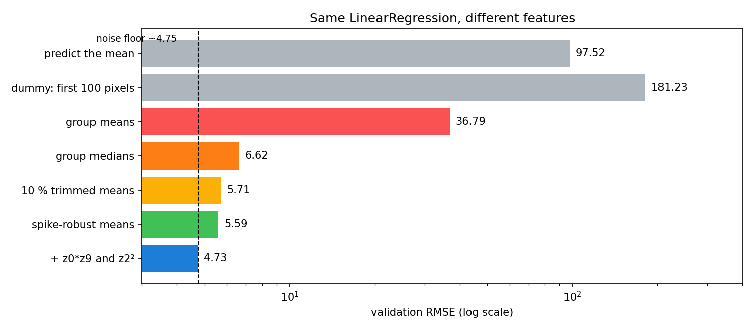
The same linear model with different features

Two results stand out. First, choosing the estimator for each group (mean versus median versus spike-robust mean) moves the RMSE from 37 to 5.6, much more than anything done afterwards. Second, gradient boosting, a far more flexible model, does worse (7.46) than linear regression on the right features: once the features are right, the problem really is linear.

What to remember

Look for structure before modelling. Correlating pixels across images revealed that 1024 "pixels" were really 10 numbers measured 100 times each. Unsupervised structure discovery is often the strongest feature engineering tool.
Averaging $n$ noisy copies divides the noise by $\sqrt n$ , but only if outliers are handled. Pick the estimator from the noise model: the mean for Gaussian noise, the median against outliers, and a mean with outlier rejection when you have both.
A linear model is as good as its features. The fit shrinks automatically for measurement noise, and a few product terms capture the interactions. Read t-statistics to keep only the terms that matter.
Estimate the noise floor. Once your error matches what the measurement noise allows (here 4.73 versus about 4.75), stop: more features or bigger models can only overfit.

"""The Mistic Alpaca (OPEIA 2025): <= 100 features + plain LinearRegression, RMSE.

Key facts found by exploration:
  * 1000 of the 1024 pixels form 10 groups of 100 pixels; inside a group every pixel is the SAME
    hidden number plus N(0, 1) noise, and about 1 % of images carry huge spikes (|x| up to 4000).
  * the value is (almost) a linear function of the 10 hidden numbers, plus z0*z9 and z2^2.
So: find the groups without labels (pixel correlations), estimate each hidden number with a
spike-robust mean, add two products, and fit LinearRegression on 12 features.

Data: the organisers' pickles (1_ml_data_start.pickle, ml_data_final_test.pickle) were converted to
.npy inside a sandbox (`python solution.py convert`); then `python solution.py` runs everything.
"""
import sys, time
import numpy as np
import pandas as pd
from scipy.sparse import csr_matrix
from scipy.sparse.csgraph import connected_components
from sklearn.linear_model import LinearRegression
from sklearn.metrics import mean_squared_error

D = 'work/'

def convert():
    """Run once, sandboxed: pickle -> .npy (never unpickle third-party files in a normal process)."""
    for fn, out in (('1_ml_data_start.pickle', 'start'), ('ml_data_final_test.pickle', 'final')):
        d = pd.read_pickle(D + fn)
        for k in d:
            for kk, v in d[k].items():
                np.save(f'{D}{out}_{k}_{kk}.npy', np.asarray(v))

def find_groups(X, n=20000, thr=0.3):
    """Unsupervised: pixels whose values are correlated across images belong to the same hidden number."""
    x = np.clip(X[:n].reshape(n, -1), -30, 100)          # clip spikes so they do not distort correlations
    sd = x.std(0)
    C = np.corrcoef(x[:, sd > 0].T)
    np.fill_diagonal(C, 0)
    _, lab = connected_components(csr_matrix(np.abs(C) > thr))
    pix = np.where(sd > 0)[0]
    groups = [pix[lab == g] for g in np.unique(lab) if (lab == g).sum() > 1]
    return sorted(groups, key=lambda g: g.min())

def latents(X, groups):
    """Spike-robust mean of each group: drop pixels more than 5 noise-sigmas from the group median."""
    X = X.reshape(len(X), -1)
    out = []
    for g in groups:
        a = X[:, g]
        ok = np.abs(a - np.median(a, 1, keepdims=True)) < 5
        out.append((a * ok).sum(1) / ok.sum(1))
    return np.stack(out, 1)

def features(Z, mu):
    Zc = Z - mu                                         # centring only makes coefficients readable
    return np.c_[Zc, Zc[:, 0] * Zc[:, 9], Zc[:, 2] ** 2]

def main():
    t0 = time.time()
    Xtr = np.load(D + 'start_X_train.npy'); ytr = np.load(D + 'start_y_train.npy')
    Xva = np.load(D + 'start_X_live_test.npy'); yva = np.load(D + 'start_y_live_test.npy')
    groups = find_groups(Xtr)
    print('groups found:', len(groups), 'sizes', sorted({len(g) for g in groups}))
    Ztr, Zva = latents(Xtr, groups), latents(Xva, groups)
    # the hidden numbers are ordered by their first pixel; map to the order used in the write-up
    mu = Ztr.mean(0)
    print('hidden-number means:', mu.round(2))
    rmse = lambda p, t: mean_squared_error(t, p) ** .5
    print('baseline, first 100 raw pixels :', round(rmse(LinearRegression().fit(Xtr.reshape(40000, -1)[:, :100], ytr)
                                                   .predict(Xva.reshape(20000, -1)[:, :100]), yva), 3))
    lin = LinearRegression().fit(Ztr, ytr)
    print('10 robust group means          :', round(rmse(lin.predict(Zva), yva), 3))
    m = LinearRegression().fit(features(Ztr, mu), ytr)
    print('12 features (+ z0*z9, z2^2)    :', round(rmse(m.predict(features(Zva, mu)), yva), 3))
    print('coefficients:', m.coef_.round(2), 'intercept', round(m.intercept_, 2))
    print(f'time so far {time.time() - t0:.1f} s')
    Xte = np.load(D + 'final_X_final_test.npy')
    pred = m.predict(features(latents(Xte, groups), mu))
    pd.DataFrame({'ID': np.arange(len(pred)), 'y_pred': pred}).to_csv('final_predictions.csv', index=False)
    print(f'final_predictions.csv written ({len(pred)} rows), total {time.time() - t0:.1f} s')

if __name__ == '__main__':
    convert() if sys.argv[1:] == ['convert'] else main()