IOAI Training: Learn AI by solving problems

The problem in brief

You must build a convolutional neural network that reads a small grey-scale photo of a face (48 x 48 pixels) and says which of seven emotions it shows: angry, disgust, fear, happy, neutral, sad or surprise. The data is the classic FER2013 dataset, given as image folders: 28 709 training faces and 7 178 test faces, each labelled by its folder. The deliverable is a notebook that trains the model and reports, on the test folder, the balanced accuracy and the macro F1-score; the statement insists on class imbalance and on robustness to hard, subtle or partly hidden expressions.

The test labels are public (they are the folder names), so we report our final numbers on the official test set. Every choice (architecture, number of epochs, the threshold correction described below) was made on a 10 % validation split carved out of the training folder; the test set was used only once per model, to report.

How you are scored

Two metrics, both insensitive to how frequent a class is. With $R_c$ the recall of class $c$ (the share of its faces that are recognised) and $P_c$ its precision:

\text{balanced accuracy} = \frac{1}{7}\sum_{c=1}^{7} R_c , \qquad \text{macro-}F_1 = \frac{1}{7}\sum_{c=1}^{7} \frac{2P_cR_c}{P_c+R_c}.

Balanced accuracy is the plain accuracy you would measure if every emotion were equally frequent. Macro F1 also punishes false alarms, through the precision. The statement gives no threshold: the submission is the reported numbers, so there is no "expected" score to compare with. For reference, plain accuracy is also reported.

First look at the data

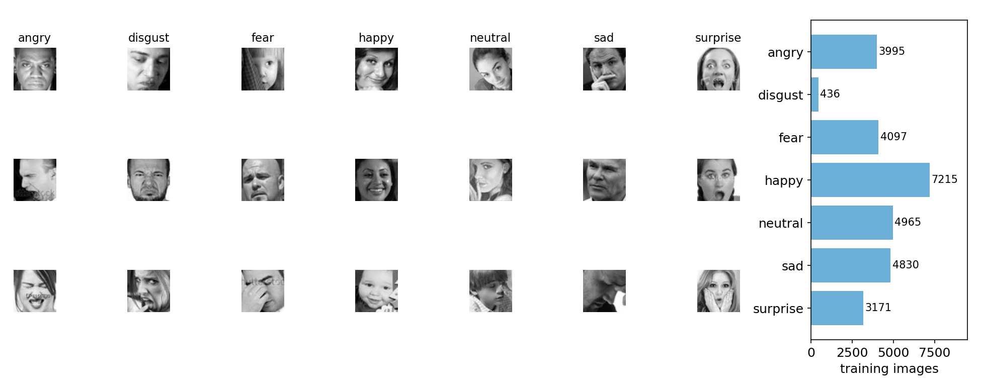
Three training faces per emotion, and the number of training faces per class

Tiny, varied images. The faces are roughly centred but vary in pose, lighting, age, glasses, hands in front of the face, and even stock-photo watermarks. Some labels are debatable (is the second "sad" face sad or thoughtful?): FER2013 is known for noisy labels, so nobody gets close to 100 %.
Strong imbalance. Happy has 7 215 training faces, disgust only 436, 16 times fewer. A model that ignores disgust loses one seventh of both metrics.
Natural confusions. Fear, surprise and sad share open eyes or mouths, and angry and disgust both frown. Expect errors there.

A first baseline

Before any network, a linear model on pixels: project the 2 304 pixel values on their first 200 principal components and fit a logistic regression. It reaches 37.3 % accuracy but only 0.299 balanced accuracy and 0.291 macro F1: it mostly predicts happy and neutral. Reweighting classes (class_weight="balanced") lifts balanced accuracy to 0.345 but costs accuracy. Pixels are a poor representation: a smile shifted by 3 pixels looks like a completely different vector.

The key idea

Two ideas do almost all the work, one for each difficulty of the task.

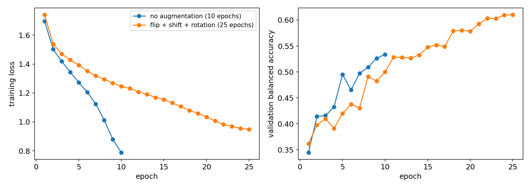
1. A CNN with data augmentation, for the images. A convolution looks for the same small pattern (an edge, a corner of the mouth) everywhere in the image, and pooling makes the answer tolerant to small shifts. That is exactly what a lopsided smile needs. But with only 26 000 training faces, a 4.7-million-parameter network memorises them quickly. Augmentation fights this: at every step each face is randomly mirrored, shifted by up to 5 %, rotated by up to 10 degrees and rescaled by up to 10 %. A mirrored smile is still a smile, so the label is unchanged, and the network sees a slightly different face each epoch. The learning curves show the effect: without augmentation the training loss falls twice as fast but validation lags behind; with augmentation the training loss stays high (the task is harder) and validation keeps improving for 25 epochs.

Training loss and validation balanced accuracy with and without augmentation

2. Logit adjustment, for the metric. A network trained with cross-entropy estimates $p(c \mid x)$ , which includes the class prior $\pi_c$ : since happy is 16 times more frequent than disgust, a borderline face is pulled towards happy. Balanced accuracy, however, is the accuracy under a uniform prior. By Bayes' rule, changing the prior from $\pi_c$ to uniform means dividing each probability by $\pi_c$ , that is subtracting $\log \pi_c$ from each log-probability:

\hat c(x) = \arg\max_c \;\big[\log p(c \mid x) - \tau \log \pi_c\big].

$\tau = 1$ is the exact Bayes correction; we choose $\tau$ on the validation split (it gives $\tau = 0.8$ , slightly under 1 because the network is a bit over-confident). No retraining is needed: it is a one-line change at prediction time. It raised the recall of disgust on the test set from 29 % to 68 %.

The full solution

Load the image folders into arrays (28 709 x 48 x 48), normalise the pixels, and keep 10 % of the training faces aside as a validation set.
Network (VGG-style): four blocks of two 3 x 3 convolutions with batch normalisation and ReLU, then max-pooling (48 to 24 to 12 to 6 to 3 pixels, 64 to 512 channels), then dropout 0.4, a 256-unit dense layer, dropout 0.4 and 7 outputs.
Training: 25 epochs of AdamW (weight decay $5 \times 10^{-4}$ , batch 128) with a one-cycle learning-rate schedule up to $2 \times 10^{-3}$ , cross-entropy with label smoothing 0.1 (useful with noisy labels), augmentation on the GPU. About 11 minutes on an Apple M-series GPU.
Test-time augmentation: average the log-probabilities of each face and of its mirror image.
Logit adjustment: subtract $0.8 \log \pi_c$ (training class shares) before the argmax.

lt = logits_of(model, x_test)                 # log-probabilities, mirror-averaged
pred = (lt - tau * np.log(prior)).argmax(1)   # tau = 0.8, chosen on validation

The adjustment is a trade-off, and the confusion matrices show it. Disgust jumps from 29 % to 68 % recall and surprise improves, while happy, angry and sad each lose a few points, because some of their faces are now given to the rare classes. Balanced accuracy, which weighs each recall equally, gains 4.3 points. Macro F1 drops slightly (0.639 to 0.626): the new disgust predictions include more false alarms, and F1 penalises the precision lost. Pick the decision rule for the metric you are judged on: use the adjusted rule for balanced accuracy, the plain argmax for macro F1.

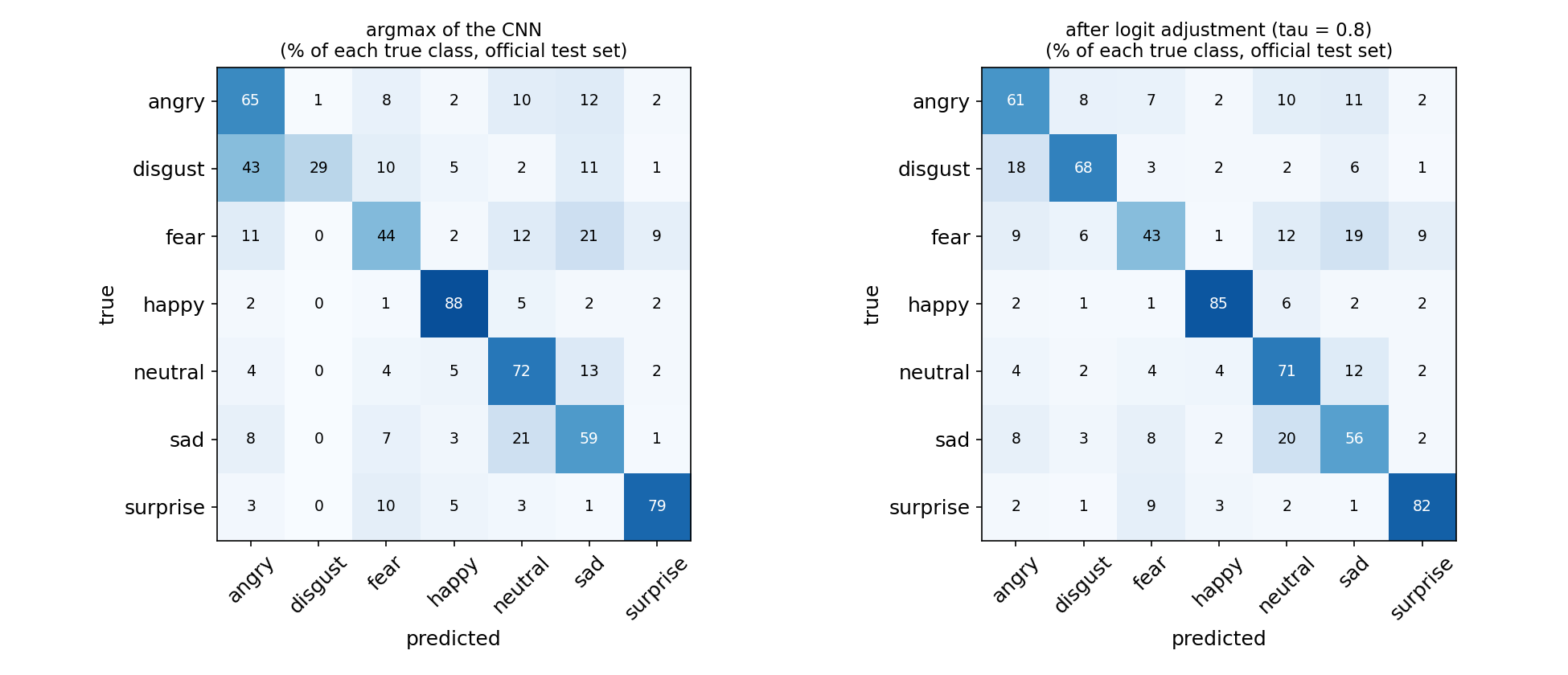
Confusion matrices on the test set before and after logit adjustment

Before the adjustment, 43 % of disgusted faces were called angry: the network had learned that a frown is "probably angry", which is true on average but not for the rare class. Fear remains the weakest emotion (43 % recall), mostly confused with sad and neutral, and a fifth of the sad faces are taken for neutral: these are the pairs that also confuse human annotators of FER2013.

Results

Official FER2013 test folder (7 178 faces); all choices made on the validation split.

approach	accuracy	balanced accuracy	macro F1
PCA-200 + logistic regression	0.373	0.299	0.291
same, class-balanced weights	0.325	0.345	0.289
CNN, no augmentation, 10 epochs	0.638	0.548	0.549
same + flip TTA + logit adjustment ( $\tau = 0.7$ )	0.638	0.621	0.579
CNN + augmentation, 25 epochs	0.681	0.612	0.626
+ flip test-time augmentation	0.691	0.624	0.639
+ logit adjustment, $\tau = 0.8$ (final for balanced accuracy)	0.679	0.667	0.626

The final model reaches 69.1 % accuracy, 0.667 balanced accuracy (with logit adjustment) and 0.639 macro F1 (without it), against 0.30 for the pixel baseline.

What to remember

Convolutions plus augmentation beat raw pixels by a mile on images: weight sharing and pooling give tolerance to small shifts, and augmentation multiplies a small dataset by encoding invariances you know are true (a mirrored face keeps its emotion).
A training loss that falls fast is not good news by itself. Compare it with the validation curve; augmentation keeps the two close and lets you train longer.
Match the decision rule to the metric. A classifier trained on imbalanced data predicts with the training prior; for balanced accuracy, subtract $\tau \log \pi_c$ from the logits (logit adjustment), with $\tau$ tuned on validation. It costs nothing and needs no retraining.
Different metrics can disagree. Logit adjustment raised balanced accuracy by 4 points but lowered macro F1 by 1: report both and know which one you optimise.
Choose on validation, report on test once. The test labels are in plain sight here; using them to pick $\tau$ or the epoch count would inflate the numbers.

"""OPEIA 2025 (Peru), "Mission EMO": 7-class facial-expression recognition on
FER2013 (48x48 grayscale), scored by balanced accuracy and macro F1 on test/.

Data: the notebook's Drive zip (id 1lBn6fRZIl7DRd2ddklw2_pIkgluv9lJi), unzipped
to work/dataset/{train,test}/<emotion>/*.jpg. Test labels are public (folders).
Model selection uses a 10 % validation split carved out of train/ only.

Usage:  python solution.py logreg | cnn_noaug | cnn       (cnn = final model, 25 epochs)
"""
import os
import sys
import time
import numpy as np
import torch
import torch.nn as nn
import torch.nn.functional as F
from PIL import Image
from sklearn.metrics import balanced_accuracy_score, f1_score, confusion_matrix

torch.set_num_threads(2)
torch.manual_seed(0); np.random.seed(0)
DEV = "mps" if torch.backends.mps.is_available() else "cpu"
ROOT = "work/dataset"
CLASSES = ["angry", "disgust", "fear", "happy", "neutral", "sad", "surprise"]


def load(split):
    cache = f"work/{split}.npz"
    if os.path.exists(cache):
        d = np.load(cache); return d["x"], d["y"]
    xs, ys = [], []
    for c, name in enumerate(CLASSES):
        folder = f"{ROOT}/{split}/{name}"
        for f in sorted(os.listdir(folder)):
            xs.append(np.array(Image.open(f"{folder}/{f}").convert("L").resize((48, 48)), dtype=np.uint8))
            ys.append(c)
    x, y = np.stack(xs), np.array(ys)
    np.savez(cache, x=x, y=y)
    return x, y


def report(name, y, pred):
    ba, f1 = balanced_accuracy_score(y, pred), f1_score(y, pred, average="macro")
    print(f"[{name}] accuracy {np.mean(pred == y):.4f}  balanced accuracy {ba:.4f}  macro F1 {f1:.4f}", flush=True)
    return ba, f1


x_all, y_all = load("train")
x_test, y_test = load("test")
rng = np.random.default_rng(0)
perm = rng.permutation(len(y_all))
n_val = len(y_all) // 10
val_idx, tr_idx = perm[:n_val], perm[n_val:]
x_tr, y_tr, x_val, y_val = x_all[tr_idx], y_all[tr_idx], x_all[val_idx], y_all[val_idx]
prior = np.bincount(y_tr, minlength=7) / len(y_tr)
print("train/val/test:", len(y_tr), len(y_val), len(y_test), "| class shares:", np.round(prior, 3))


# ------------------------------------------------------------------ model
def block(cin, cout):
    return nn.Sequential(nn.Conv2d(cin, cout, 3, padding=1, bias=False), nn.BatchNorm2d(cout), nn.ReLU(inplace=True),
                         nn.Conv2d(cout, cout, 3, padding=1, bias=False), nn.BatchNorm2d(cout), nn.ReLU(inplace=True),
                         nn.MaxPool2d(2))


class Net(nn.Module):            # VGG-style: 48 -> 24 -> 12 -> 6 -> 3, about 4.7 M parameters
    def __init__(self):
        super().__init__()
        self.features = nn.Sequential(block(1, 64), block(64, 128), block(128, 256), block(256, 512))
        self.head = nn.Sequential(nn.Flatten(), nn.Dropout(0.4), nn.Linear(512 * 9, 256), nn.ReLU(inplace=True),
                                  nn.Dropout(0.4), nn.Linear(256, 7))

    def forward(self, x):
        return self.head(self.features(x))


def augment(xb):
    """Random horizontal flip, shift (up to 5 %), rotation (up to 10 degrees) and scale (up to 10 %), on the GPU."""
    n = xb.shape[0]
    flip = torch.rand(n, device=xb.device) < 0.5
    xb = torch.where(flip[:, None, None, None], xb.flip(3), xb)
    ang = (torch.rand(n, device=xb.device) - 0.5) * 2 * np.deg2rad(10)
    sc = 1 + (torch.rand(n, device=xb.device) - 0.5) * 0.2
    tx, ty = [(torch.rand(n, device=xb.device) - 0.5) * 0.2 for _ in range(2)]
    theta = torch.stack([torch.stack([torch.cos(ang) / sc, -torch.sin(ang) / sc, tx], 1),
                         torch.stack([torch.sin(ang) / sc, torch.cos(ang) / sc, ty], 1)], 1)
    grid = F.affine_grid(theta, xb.shape, align_corners=False)
    return F.grid_sample(xb, grid, padding_mode="border", align_corners=False)


def to_tensor(x):
    return ((torch.tensor(x, dtype=torch.float32) / 255.0 - 0.5) / 0.25).unsqueeze(1)


@torch.no_grad()
def logits_of(model, x, tta=True):
    model.eval()
    out = []
    for k in range(0, len(x), 512):
        xb = to_tensor(x[k:k + 512]).to(DEV)
        z = F.log_softmax(model(xb), 1)
        if tta:                                      # average with the mirrored face
            z = (z + F.log_softmax(model(xb.flip(3)), 1)) / 2
        out.append(z.cpu())
    return torch.cat(out).numpy()


def train_cnn(epochs, aug, lr=2e-3, bs=128):
    model = Net().to(DEV)
    opt = torch.optim.AdamW(model.parameters(), lr=lr, weight_decay=5e-4)
    steps = epochs * (len(y_tr) // bs)
    sched = torch.optim.lr_scheduler.OneCycleLR(opt, max_lr=lr, total_steps=steps, pct_start=0.2)
    X, Y = to_tensor(x_tr), torch.tensor(y_tr)
    hist = []
    for ep in range(epochs):
        model.train()
        p = torch.randperm(len(Y))
        tot = 0
        for k in range(0, len(Y) - bs + 1, bs):
            xb, yb = X[p[k:k + bs]].to(DEV), Y[p[k:k + bs]].to(DEV)
            if aug:
                xb = augment(xb)
            loss = F.cross_entropy(model(xb), yb, label_smoothing=0.1)
            opt.zero_grad(); loss.backward(); opt.step(); sched.step()
            tot += loss.item()
        pv = logits_of(model, x_val, tta=False).argmax(1)
        hist.append((tot / (len(Y) // bs), balanced_accuracy_score(y_val, pv)))
        print(f"  epoch {ep + 1}/{epochs} train loss {hist[-1][0]:.3f} val balanced acc {hist[-1][1]:.4f}", flush=True)
    return model, hist


if __name__ == "__main__":
    mode = sys.argv[1] if len(sys.argv) > 1 else "cnn"
    t0 = time.time()
    if mode == "logreg":                       # pixel-level linear baseline
        from sklearn.linear_model import LogisticRegression
        from sklearn.decomposition import PCA
        pca = PCA(200, random_state=0).fit(x_tr.reshape(len(x_tr), -1) / 255.0)
        f = lambda x: pca.transform(x.reshape(len(x), -1) / 255.0)
        clf = LogisticRegression(max_iter=2000, C=1.0).fit(f(x_tr), y_tr)
        report("PCA-200 + logistic regression, test", y_test, clf.predict(f(x_test)))
        clf_b = LogisticRegression(max_iter=2000, C=1.0, class_weight="balanced").fit(f(x_tr), y_tr)
        report("same, class_weight=balanced, test", y_test, clf_b.predict(f(x_test)))
    elif mode in ("cnn_noaug", "cnn"):
        epochs, aug = (10, False) if mode == "cnn_noaug" else (25, True)
        model, hist = train_cnn(epochs, aug)
        np.save(f"work/hist_{mode}.npy", np.array(hist))
        lv, lt = logits_of(model, x_val), logits_of(model, x_test)
        report(f"{mode}, test, no TTA", y_test, logits_of(model, x_test, tta=False).argmax(1))
        report(f"{mode}, test, flip TTA", y_test, lt.argmax(1))
        # Post-hoc logit adjustment: balanced accuracy is the accuracy under a UNIFORM
        # class prior, so subtract tau * log(train prior); tau chosen on validation only.
        taus = np.linspace(0, 1.5, 16)
        bas = [balanced_accuracy_score(y_val, (lv - t * np.log(prior)).argmax(1)) for t in taus]
        tau = taus[int(np.argmax(bas))]
        print(f"validation balanced acc vs tau: {dict(zip(np.round(taus, 1), np.round(bas, 4)))} -> tau = {tau:.1f}")
        pred = (lt - tau * np.log(prior)).argmax(1)
        report(f"{mode}, test, flip TTA + logit adjustment", y_test, pred)
        np.save(f"work/cm_{mode}.npy", confusion_matrix(y_test, pred))
        np.save(f"work/cm_{mode}_raw.npy", confusion_matrix(y_test, lt.argmax(1)))
    print(f"done in {(time.time() - t0) / 60:.1f} min")

AI Challenge: Mission EMO — Teaching Machines to Feel