IOAI Training: Learn AI by solving problems

The problem in brief

You receive a Qwen3.5-2B language model with three parts cut off: the embedding table, the first decoder layer and the output head. Only layers 1 to 23 and the final normalisation are left. For each of 1 000 multiple-choice questions (a context, a question, four options A to D plus two "sink" options that are never right) you get the hidden states right after layer 0, one 2048-dimensional vector per token, and the positions of the end-of-line token of each of the four options. You cannot read the text, you cannot feed new text, and you cannot ask the model for the letter of its answer. You must still pick the right option. 100 extra questions come with their answer.

The data comes from the Kaggle competition archive. The labels of the 1 000 questions are private and we never submitted anything, so all scores below are 5-fold cross-validation on the 100 labelled questions (repeated 4 times). With 100 questions the standard error is about $\pm 4$ points, so differences of 1 or 2 points mean nothing.

How you are scored

Accuracy over the 1 000 questions: the fraction where your option index (0 to 3) is the correct one. Chance is 25 %.

What to aim for. The organisers' "author solution" scores 0.780 on the public leaderboard; the best contestants reach 0.765 and 0.763.

First look at the data

The questions are 88 to 337 tokens long. Two engineering facts shape everything:

The model does not fit our budget. The 23 layers are 2.4 GB in bfloat16 and twice that in float32, and the machine allows 3 GB per process.
The pickles are third-party files, so we open them only inside a sandbox and convert them to plain arrays: one fp16 matrix with all tokens of all questions, plus offsets, option positions and labels.

The layer-0 states already reveal the prompt template. After removing the mean vector (all states share a large common direction), the same token has almost the same state in every question: the token right after each option's end-of-line has cosine 0.99 across questions (it is the next option's letter), and the last 19 tokens of every prompt are identical (the sink options and the answer cue). This lets us locate the letters A to D, but it does not give us the output head, so it does not directly give the answer.

A first baseline

The organisers' baseline runs the stripped model to the end, takes the final-layer state at the end of each option, and trains a logistic regression "is this option the right one?" on the 100 labelled questions; the option with the highest score wins. In our cross-validation this gives 0.355. The same probe on the raw layer-0 states gives 0.31. Both are close to chance.

We also tried a zero-shot "letter lens": the output head of Qwen is tied to its embedding table, so the logit of letter $k$ is the final normalised last-position state dotted with that letter's embedding, and we approximated the embedding by the layer-0 state at the letter's position. It gave 0.21 to 0.26: the layer-0 state is too far from the pure embedding, and the answer is probably generated as a different token (with a leading space).

The key idea

Read the answer from the middle of the network, not from its end. We probed the state at the end of each option after every layer:

Probe accuracy layer by layer

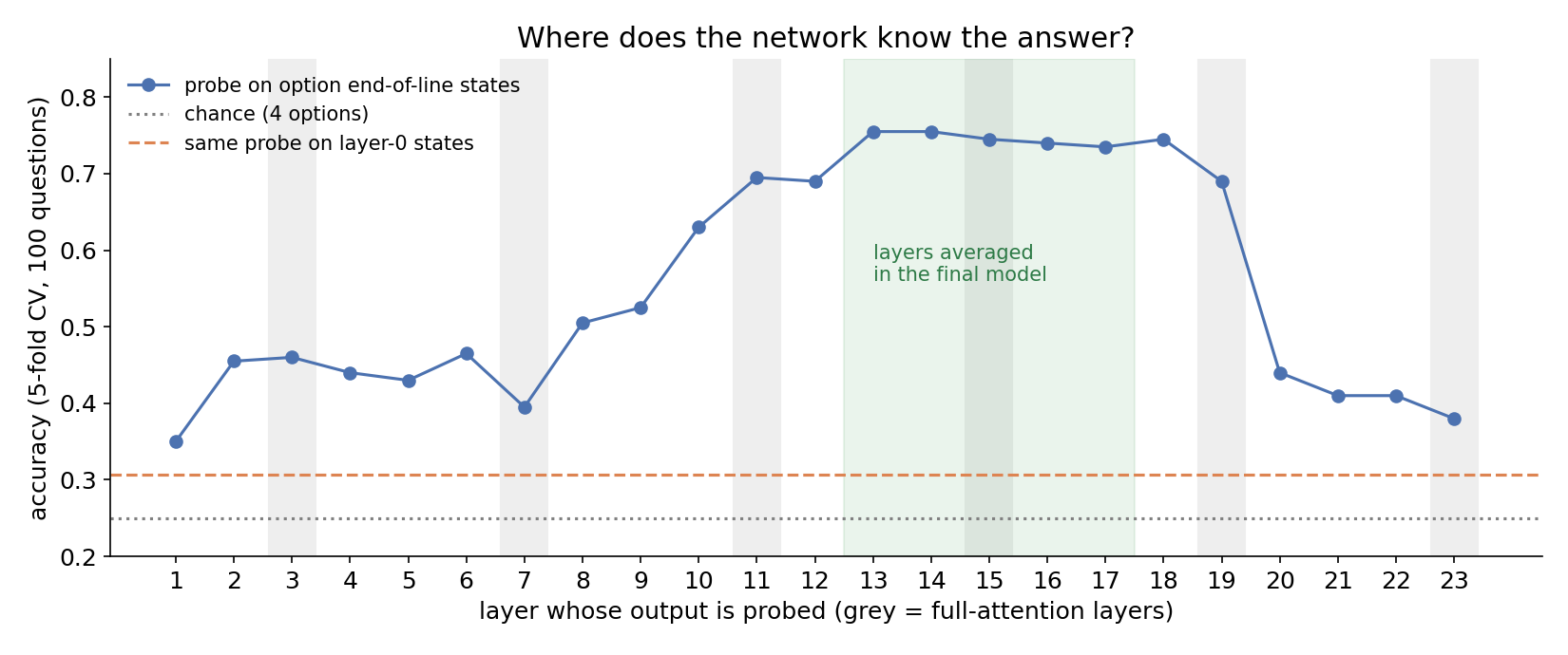
The curve tells a clear story. Early layers (1 to 9) hold little more than the tokens (40 to 50 %). From layer 10 the accuracy climbs fast and reaches 0.75 at layers 13 and 14: by then the network has read the question and each option, and the end-of-line token of the right option is represented differently from the others. Then the accuracy collapses after layer 19, down to 0.38 at layer 23. The last layers are busy preparing the next-token prediction (they turn "option C is right" into "the next token is C") and that information lives at the last position of the prompt and in the output vocabulary, which we do not have. This is a well-known pattern of transformers: the most linearly decodable, task-general features sit in the middle layers, and the last layers specialise in the output format.

The second idea is purely practical: stream the layers. Instead of loading the model, we keep the hidden states of 100 questions in memory and apply one layer at a time, loading it from disk, then the next:

for L in range(1, 20):                      # layers outside, questions inside
    tm.layers[L] = load_layer(L)            # ~110 MB in bfloat16, float32 on the GPU
    for j, q in enumerate(questions):
        H[j] = tm(inputs_embeds=H[j][None]).last_hidden_state[0]
    tm.layers[L] = Pass()                   # free it before loading the next one

All other layers are identity modules, so the model's own code still builds the masks and rotary embeddings. Peak memory stays under 3 GB and the whole forward pass for 1 100 questions takes about 6 minutes. One more trick keeps memory flat on the Apple GPU: we pad every sequence on the right to a multiple of 64 tokens. The model is causal, so padding after the last token cannot change any earlier state (we checked: the states match the unpadded run to fp16 precision).

The full solution

In the sandbox, convert the pickles to .npy and split model.pt into one safetensors file per layer.
Stream layers 1 to 19 over the 1 100 questions (100 at a time), keeping the four option end-of-line states after each layer.
For each of the layers 13 to 17, standardise the features and fit a logistic regression with strong L2 regularisation ( $C = 0.05$ , because 100 questions give only 400 examples in 2048 dimensions). Each option gets a score per layer.
Sum the five scores and answer with the best option. For the submission the probes are fitted on all 100 labelled questions.

Results

5-fold cross-validation on the 100 labelled questions, repeated 4 times (official labels private).

approach	accuracy
chance	0.25
zero-shot letter lens (layer-0 letter states as output head)	0.21 to 0.26
probe on layer-0 states	0.31
probe on final-layer states, final norm (organisers' baseline)	0.355
probe on layer 7 / layer 10	0.395 / 0.630
probe on layer 13 (best single layer)	0.755
probe on layer 13, features centred within each question	0.745
sum of probes on layers 13 to 17 (final)	0.748
same, standardised with the 1 000 unlabelled questions too	0.748
same + self-training on pseudo-labelled questions	0.720 to 0.725

The final model reaches 0.75 in cross-validation, versus 0.36 for the baseline and 0.78 for the author solution on the leaderboard; with $\pm 4$ points of uncertainty on our estimate, we cannot tell whether it is truly below the author's. Averaging five neighbouring layers is not better than the best single layer in cross-validation, but it is more robust than picking a layer from a noisy 100-question curve. Self-training (adding the confident predictions on the unlabelled questions as training data) hurt by 2 to 3 points: with a probe that is wrong a quarter of the time, pseudo-labels add as much noise as signal.

What to remember

Probe every layer. The last layer of a language model is not the best representation for a new task; the middle layers often are. A 20-line loop over layers turned 0.36 into 0.75.
A missing head does not mean missing knowledge. The decision is computed inside the network long before the output layer; a linear probe trained on a few labelled examples can read it.
Models can be run layer by layer. When weights do not fit in memory, move the loop over layers outside the loop over inputs and keep only activations in memory.
Use causality. Right padding is free in a causal model, and fixed shapes keep GPU memory under control.
With 100 labels, regularise hard and distrust small gains. Strong L2, few hyperparameters, repeated cross-validation, and an honest error bar.

"""CutiesNLP (NEOAI 2026, day 2): multiple choice with a stripped Qwen3.5-2B.

We only have layers 1-23 + final norm (no embedding table, no layer 0, no LM head) and,
for every question, the hidden states after layer 0. Plan:
  1. (sandbox) unpickle the third-party files and convert them:
       student_*.pkl -> <split>_emb.npy (all tokens, fp16) + <split>_meta.npz (offsets, option positions, labels)
       model.pt      -> layers/layerNN.safetensors (one file per decoder layer)
  2. continue the forward pass on our own machine, 100 questions at a time and ONE layer
     in memory at a time (the full model does not fit in a 3 GB budget), keeping the
     hidden state at the end-of-line token of each of the 4 options for layers 1..19;
  3. a logistic "probe" per middle layer (13..17) scores each option, trained on the 100
     labelled questions; the 5 scores are summed and the best option is the answer.

Data: kaggle competition "neoai-2026-day-2-cutiesnlp".
Usage: run_sandboxed.sh . python3 solution.py convert      (unpickling step, no network)
       python3 solution.py forward student_train ; python3 solution.py forward student_val
       python3 solution.py fit                              (CV score + submission.csv, not submitted)
Runtime: ~6 min forward on Apple MPS for 1 100 questions; peak memory ~2.9 GB.
"""
import os, sys, pickle, time, numpy as np, torch, torch.nn as nn
from safetensors.torch import load_file, save_file
from sklearn.linear_model import LogisticRegression
from sklearn.model_selection import RepeatedKFold

LAYERS, C = [13, 14, 15, 16, 17], 0.05


def convert():
    for split in ['student_train', 'student_val']:
        d = pickle.load(open(f'{split}.pkl', 'rb'))
        off = np.cumsum([0] + [len(x['embeds_after_l0']) for x in d])
        E = np.lib.format.open_memmap(f'{split}_emb.npy', 'w+', np.float16, (int(off[-1]), 2048))
        for x, o in zip(d, off):
            E[o:o + len(x['embeds_after_l0'])] = x['embeds_after_l0']
        E.flush()
        np.savez(f'{split}_meta.npz', off=off, idx=np.array([x['idx'] for x in d]),
                 eol=np.array([x['eol_positions'] for x in d]), y=np.array([x.get('correct_idx', -1) for x in d]))
    sd = torch.load('model.pt', map_location='cpu', weights_only=True, mmap=True)
    os.makedirs('layers', exist_ok=True)
    for L in range(1, 24):
        save_file({k: v.contiguous().clone() for k, v in sd.items() if k.startswith(f'model.layers.{L}.')},
                  f'layers/layer{L:02d}.safetensors')


def forward(split, lmax=19):
    from transformers import Qwen3_5TextConfig
    from transformers.models.qwen3_5.modeling_qwen3_5 import (Qwen3_5TextModel, Qwen3_5DecoderLayer,
                                                              Qwen3_5TextRotaryEmbedding)
    torch.set_num_threads(2)
    dev = 'mps' if torch.backends.mps.is_available() else 'cpu'
    if dev == 'mps':
        torch.mps.set_per_process_memory_fraction(0.08)

    class Pass(nn.Module):
        def forward(self, x, *a, **k): return x

    cfg = Qwen3_5TextConfig.from_pretrained('model_config')
    with torch.device('meta'):                       # skeleton only: no weights allocated
        tm = Qwen3_5TextModel(cfg)
    tm.embed_tokens, tm.norm = nn.Identity(), nn.Identity()
    tm.rotary_emb = Qwen3_5TextRotaryEmbedding(cfg).to(dev)
    tm.layers = nn.ModuleList([Pass() for _ in range(cfg.num_hidden_layers)])
    m = np.load(f'{split}_meta.npz'); off = m['off']; nq = len(off) - 1
    E = np.load(f'{split}_emb.npy', mmap_mode='r')
    out = {L: np.zeros((nq, 4, 2048), np.float16) for L in range(1, lmax + 1)}

    def padded(q):   # right padding cannot affect earlier positions in a causal model; fixed shapes for MPS
        a = np.asarray(E[off[q]:off[q + 1]], np.float32); P = 64 * ((len(a) + 63) // 64)
        return torch.from_numpy(np.concatenate([a, np.zeros((P - len(a), 2048), np.float32)]))

    for c0 in range(0, nq, 100):
        qs = range(c0, min(nq, c0 + 100)); H = [padded(q) for q in qs]
        for L in range(1, lmax + 1):                  # the layer loop is OUTSIDE the question loop
            layer = Qwen3_5DecoderLayer(cfg, L)
            layer.load_state_dict({k.split(f'model.layers.{L}.', 1)[1]: v
                                   for k, v in load_file(f'layers/layer{L:02d}.safetensors').items()})
            tm.layers[L] = layer.to(dev, torch.float32).eval()
            with torch.no_grad():
                for j, q in enumerate(qs):
                    x = H[j].to(dev)[None]
                    h = tm(inputs_embeds=x, attention_mask=torch.ones(1, x.shape[1], dtype=torch.long, device=dev),
                           use_cache=False).last_hidden_state[0].cpu()
                    H[j] = h; out[L][q] = h[m['eol'][q]].numpy().astype(np.float16)
            tm.layers[L] = Pass(); del layer
            if dev == 'mps':
                torch.mps.empty_cache()
        print(f'{split}: questions up to {qs[-1]} done', flush=True)
    np.savez(f'feat_{split}.npz', **{f'L{L:02d}': v for L, v in out.items()})


def probe_scores(Ftr, ytr, Fte):
    """One pointwise logistic probe per layer ('is this option correct?'), scores summed over layers."""
    S = 0
    for L in LAYERS:
        A, B = Ftr[f'L{L:02d}'].astype(np.float32), Fte[f'L{L:02d}'].astype(np.float32)
        X = A.reshape(-1, 2048); mu, sd = X.mean(0), X.std(0) + 1e-6
        lab = (np.arange(4)[None] == ytr[:, None]).reshape(-1)
        clf = LogisticRegression(C=C, max_iter=3000).fit((X - mu) / sd, lab)
        S = S + clf.decision_function(((B - mu) / sd).reshape(-1, 2048)).reshape(len(B), 4)
    return S


if __name__ == '__main__':
    if sys.argv[1] == 'convert':
        convert()
    elif sys.argv[1] == 'forward':
        forward(sys.argv[2])
    else:
        ft = dict(np.load('feat_student_train.npz')); fv = dict(np.load('feat_student_val.npz'))
        y = np.load('student_train_meta.npz')['y']
        accs = []
        for tr, te in RepeatedKFold(n_splits=5, n_repeats=4, random_state=0).split(y):
            S = probe_scores({k: v[tr] for k, v in ft.items()}, y[tr], {k: v[te] for k, v in ft.items()})
            accs.append((S.argmax(1) == y[te]).mean())
        print(f'5-fold CV accuracy on the 100 labelled questions: {np.mean(accs):.3f}')
        pred = probe_scores(ft, y, fv).argmax(1)
        idx = np.load('student_val_meta.npz')['idx']
        np.savetxt('submission.csv', np.c_[idx, pred], fmt='%d', delimiter=',', header='id,target', comments='')
        print('wrote submission.csv (not submitted); class counts', np.bincount(pred))