IOAI Training: Learn AI by solving problems

The problem in brief

The IOAI logo is described as a function $F(x, y)$ on a rectangle of the plane, with five regions. In the first letter I the field is a linear gradient. In the O it follows a spiral pattern. In the A it is the constant $-1$ . In the last I it must be random, and the randomness may only come from nn.Dropout. Everywhere else it is $0$ . Hidden parameters change the pose of each letter (angle, scale, thickness). You must train from scratch a PyTorch model with fewer than 20,260 parameters that reproduces the field. During the contest you could sample the official generator as much as you liked. At grading time your notebook was re-run on hidden configurations, and the model was scored region by region.

What we could actually evaluate. The official generator is shipped only as obfuscated binaries for Linux x86-64 and CPython 3.13, which cannot run on our machine (no Linux container available). The organisers' Hugging Face dataset, however, contains sampled fields from the same family: 40 training fields (3000 labelled points each) and 8 held-out fields, each with 2500 labelled context points and 6000 query points whose values and region ids are in the private part. In these files the first I ranges from about $-16$ to $16$ , not $10^{10}$ and more as in the contest configs. We therefore solve the closest scorable version: for each held-out field, train a model on its 2500 context points only, then score it on its 6000 query points with the official region formulas. This is harder than the contest on one side (2500 points instead of unlimited sampling), and easier on the other (smaller values in the first I). The scores below are not comparable to the contest leaderboard.

How you are scored

For the first I, the O and the A, the score is a normalised mean absolute error:

\mathrm{score}(R) = 1 - \min\!\left(\frac{\mathrm{MAE}(R)}{s_R},\, 1\right),

where $s_R$ is the spread between the 1st and 99th percentiles of the true values in the region (1 if the region is constant, as for A). For the background the scale is fixed and tiny, $s_{bg} = 0.1$ . For the last I, the grader turns dropout on, runs the model $K = 10$ times, and gives each point $\min(\sigma_j / s_E, 1)$ with $s_E = \sqrt{1/12} \approx 0.29$ . A point scores 0 if any of its 10 outputs leaves $[-2026, 2026]$ . The total is $100\times$ the mean of the five region scores, and it is halved if the model has 20,260 parameters or more.

Contest reference points (statement): the official baseline scored 31.22 and the Scientific Committee 63.53 on the real task. In the official results table, the second-best contestant has 71.4 and the median is 14.2; the table's maximum is exactly 100, apparently rescaled to the best contestant. In our sampled-field version, predicting the constant 0 everywhere already scores 46.8, because the first I is centred on zero there.

First look at the data

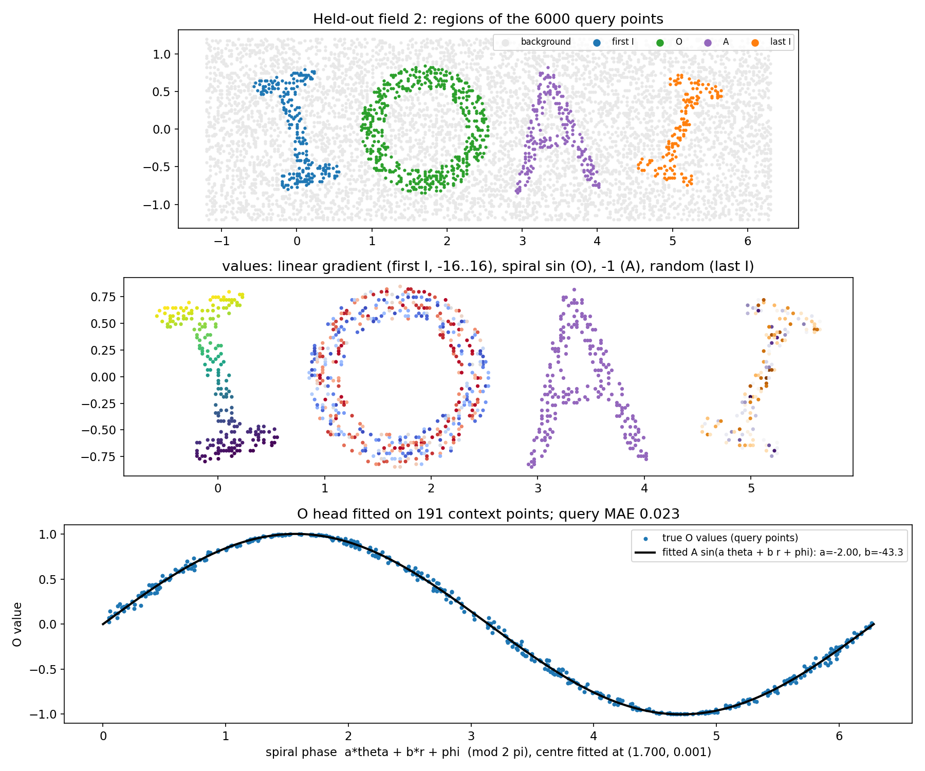
Held-out field 2. Top: the regions of the 6000 query points. Middle: the values. Bottom: the O values plotted against the phase of the fitted spiral.

Three observations decide everything.

The letters are thin strokes, and the first I has serifs, so it is not convex. Our first geometric idea, "the first I is the convex hull of its points", was wrong and made things worse (see Results).
The metric is very asymmetric. In the background the scale is $0.1$ . A single background point predicted at value 10 (inside the first I's gradient) adds $10/(0.1\,N_{bg})$ to the normalised error. With 512 background points that is 20 % of the background score, and in the contest, where the first I is worth $10^{10}$ , it costs the whole region. A point of the first I predicted as 0 costs at most $|v|/(s_I N_I)$ : little, especially near the middle of the gradient where $v \approx 0$ .
The O is an exact formula. Plotted in polar coordinates around the ring's centre, the O values are $\sin(a\theta + b r + \varphi)$ with $a = \pm 2$ and $|b| \approx 43$ : a two-armed spiral. The catch is that the centre must be very precise. The mean of the O points is off by about 0.05, and with $b \approx 43$ that shifts the phase by about 2 radians, which destroys the fit.

Labels for the context points. The context points carry values, not region ids, but the regions can be read off the values: $v = 0$ is background, $v = -1$ is the A, and the remaining points split into three spatial groups (single-linkage clustering), ordered left to right as first I, O and last I.

A first baseline

The hinted architecture is a router plus heads. A small MLP classifies each point into one of the five regions; a hard argmax picks the head; each region has its own small head:

first I: nn.Linear(2, 1) fitted by least squares (the gradient is exactly linear: residual $3\times10^{-7}$ );
O: a small MLP on polar features around the centroid of the O points;
A: the constant $-1$ ;
last I: $1000\cdot(\mathrm{dropout}(1) - 1)$ , which is $0$ in eval mode and $\pm1000$ in train mode;
background: $0$ .

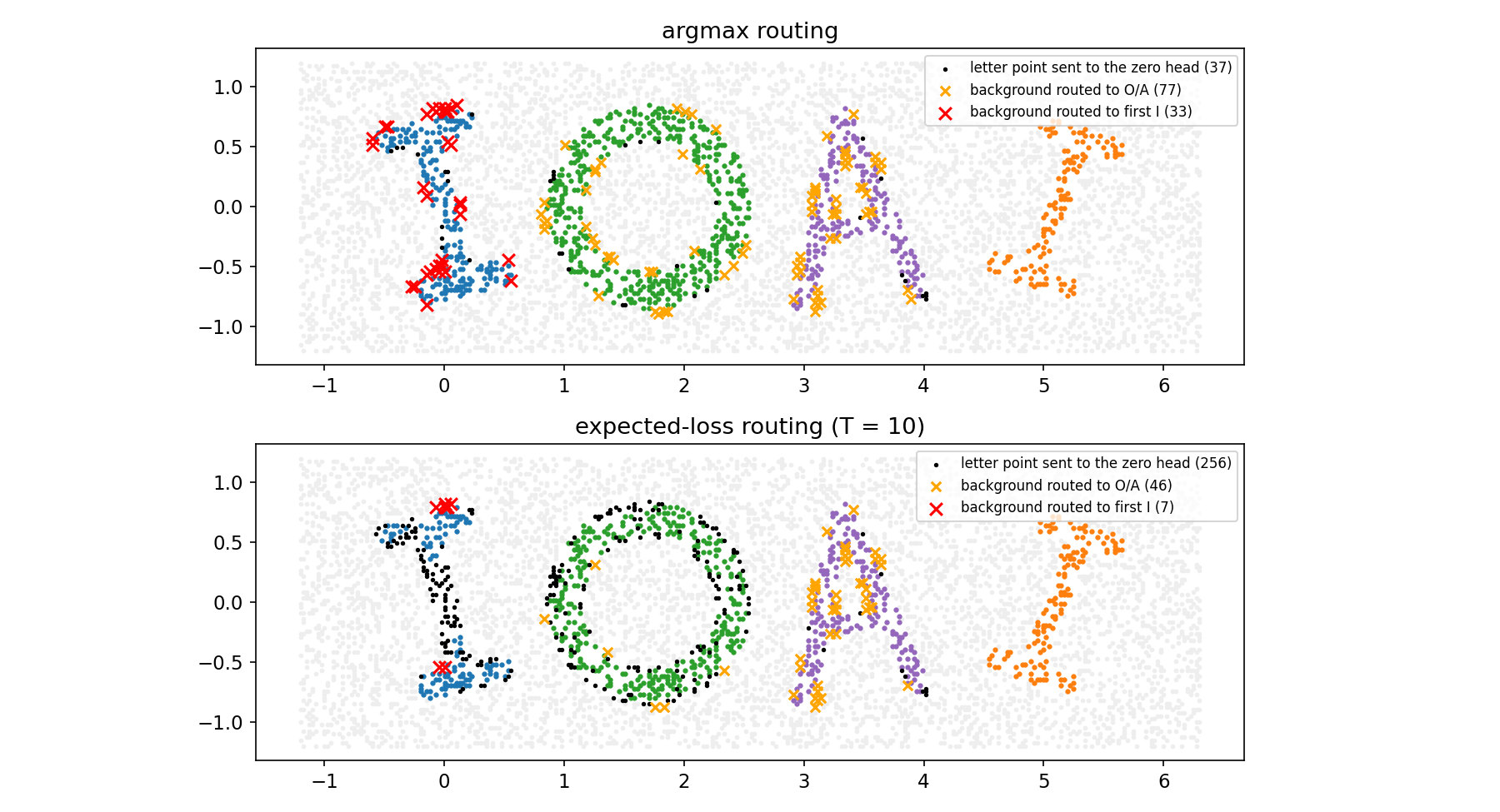
The router is an MLP ( $2 \to$ 16 random Fourier features $\to 64 \to 64 \to 5$ , GELU), trained with class-balanced cross-entropy on the 2500 context points. The whole model has 8,118 parameters. Mean over the 8 held-out fields: 76.5. The regions are classified with 97 % accuracy, and the first I scores 0.97, but the background scores only 0.20. The diagnosis (top panel of the next figure): about 30 background points per field are routed to the first I, just outside its strokes, and each one carries a large linear-gradient value.

The key idea

The router should not choose the most probable region. It should choose the output that costs the least score in expectation. Let $p_j(x)$ be the router's probability (with class-balanced training, so it matches the grader's equal number of points per region), $\hat y_k(x)$ the output if we route to $k$ , and $y_j(x)$ the value the field would have if the point belonged to $j$ (given by the heads: linear gradient, spiral, $-1$ , $0$ ). Route to

k^\star(x) = \arg\min_k \sum_j p_j(x)\, c_{jk}(x),

where each cost is the normalised error in that region's own units, capped at 1:

c_{jk} = \min\!\left(\frac{|\hat y_k - y_j|}{s_j}, 1\right)\ \ (j \in \{I, O, A\}), \qquad c_{bg,k} = \min\!\left(\frac{|\hat y_k|}{0.1}, 1\right).

The last I adds a cost of 1 for every choice except the last-I head. This is plain Bayes decision theory: minimise the expected loss instead of the expected error rate. The router's probabilities are overconfident, so we soften them with a temperature, $p = \mathrm{softmax}(z/T)$ ; $T = 10$ was chosen on the training fields, never on the held-out ones.

Two consequences, both visible in the figure below.

Near the middle of the first I, routing to "zero" wins. There $|v|$ is small compared with $s_I$ , so predicting 0 costs almost nothing, while a background point predicted on the gradient would cost a lot. Expected-loss routing gives up the cheap points of the I and protects the background: background points routed to the first I fall from 33 to 7 on this field.
The last-I head is free for the background. Its eval-mode output is exactly 0, the right background value, and its noise only appears in train mode, which the grader uses only on last-I points. So every uncertain point can go to the noise head: it is correct if it is background and full score if it is the last I. The last-I score jumps to 0.998.

Routing on held-out field 2. Top: argmax of the router. Bottom: expected-loss routing. Red crosses are background points routed to the first I, the most expensive error; black dots are letter points sent to a zero-valued head, a cheap error.

Second idea: an exact formula beats a network when you can find it. We replace the O network with a 6-parameter head $A\sin(a\,\mathrm{atan2}(y - c_y, x - c_x) + b\,\lVert (x, y) - c\rVert + \varphi)$ . Its centre $c$ is learned, and it is fitted by L1 regression (the metric is an MAE) from 96 starting points ( $a \in \{\pm1, \pm2, \pm3\}$ , $b \in \{\pm 40, \pm 45\}$ , 4 phases), 300 Adam steps each. On field 2 it finds $a = -2.00$ , $b = -43.3$ , centre $(1.700, 0.001)$ , and a query MAE of 0.023 from only 191 points.

The full solution

Labels: derive the region ids of the 2500 context points from their values (0, $-1$ , three clusters ordered by $x$ ).
Router: an MLP on fixed random Fourier features (stored as non-trainable nn.Parameters, because the grader forbids buffers), trained 2000 Adam steps with class-balanced cross-entropy.
First I head: a linear layer set by least squares on the first-I context points.
O head: the spiral formula, fitted by multi-start L1 regression with a learnable centre.
A, background, last I: the constant $-1$ , zero, and $1000(\mathrm{dropout}_{0.5}(1) - 1)$ .
Routing at inference: expected-score-loss decision with $T = 10$ , using the heads' own outputs as the candidate values.

p = torch.softmax(self.logits(xy) / self.temp, 1)
yi, yo = self.heads(xy)                                   # gradient and spiral at every point
outs = torch.stack([yi, yo, -ones, zeros, zeros], 1)      # eval-mode output of each choice
cost = p[:, BG:BG+1] * (outs.abs() / 0.1).clamp(max=1)    # background truth
for j, (truth, s) in enumerate([(yi, s_I), (yo, s_O), (-ones, 1.0)]):
    cost += p[:, j:j+1] * ((outs - truth[:, None]).abs() / s).clamp(max=1)
cost += p[:, E:E+1] * miss_e                              # last I: lose 1 unless routed to the noise head
reg = cost.argmin(1)

Everything is plain torch inside one nn.Module with 8,118 parameters, deterministic in eval mode, with randomness only from nn.Dropout. Fitting one field takes about 15 s on two CPU threads.

Results

Mean over the 8 held-out fields, each model trained on that field's 2500 context points and scored on its 6000 query points (official region formulas; query values and regions from private/test_private.npz). Tuning (bias, temperature) was done only on 8 training fields, split 2500/500.

approach	first I	O	A	bg	last I	total
constant 0 everywhere				1.00	0	46.8
constant $-1$ everywhere			1.00	0	0	42.9
router (argmax) + linear I + MLP O	0.974	0.776	0.940	0.201	0.932	76.5
same + background logit bias 5 (crude conservatism)	0.941	0.774	0.832	0.668	0.813	80.6
first I = convex hull of its points (failed: the I has serifs)	0.909	0.757	0.960	0.000	0.934	71.2 (train fields)
argmax + spiral O	0.974	0.948	0.940	0.214	0.932	80.2
expected-loss routing ( $T = 10$ ) + MLP O	0.862	0.764	0.913	0.811	0.998	86.9
expected-loss routing + spiral O (final, `solution.py`)	0.881	0.912	0.914	0.784	0.998	89.8

The two ideas stack up: the spiral helps the O, expected-loss routing helps the background and the last I, and together they turn 76.5 into 89.8. The remaining loss is mostly background points routed to the A or the O near their strokes (46 on field 2): with 2500 random points the strokes' edges are only known to within about 0.04.

How this transfers to the real contest. With unlimited samples from the generator, the router can be trained on millions of points, so its boundaries become far sharper than with 2500 points. With values of $10^{10}$ in the first I, our capped per-point cost understates the danger: any background point routed to the first I zeroes the whole background region. A contestant should then forbid that routing unless the router is near-certain (in practice, a very low temperature on the first I only, or an eroded I mask), and normalise the linear head by i_grad_min/i_grad_max from the config file. We could not verify these numbers without the official runtime, so we make no claim against the 63.53 of the Scientific Committee.

What to remember

Decide with the metric, not with the argmax. When errors have very different costs, choose $\arg\min_k \sum_j p_j c_{jk}$ . Here this made the model give up cheap points of the I to protect the expensive background.
Read how the grader uses each mode. The noise head's output is 0 in eval mode and random only in train mode, which the grader uses only on the last I. Treating it as the "background or last I" head was worth several points, entirely within the rules.
Look for the formula. A 6-parameter spiral, fitted with a learnable centre and multiple starts, beat a neural head trained on the same 150 points (O score from 0.78 to 0.91). Small parameter budgets reward structure, not width.
Check geometric assumptions on a picture first. The convex-hull idea looked elegant and failed, because the I has serifs.
Tune on training fields, report on held-out ones. The temperature was chosen on the training fields; the held-out score came out within 2 points of the training-field estimate (89.8 against 92.0).

"""IOAI Field on the organisers' sampled fields (official generator is platform-locked).
For each of the 8 held-out fields: fit a <20,260-parameter torch model on the 2500 context points,
score it on the 6000 query points (private values + region ids) with the official region formulas.
Final recipe (defaults): class-balanced MLP router on Fourier features, exact least-squares linear head
for the first I, parametric spiral head A sin(a*theta + b*r + phi) with a learnable centre for O,
constant -1 for A, dropout noise for the last I, and EXPECTED-SCORE-LOSS routing (temperature 10)
instead of argmax. Usage: python solution.py [bg_bias] [steps] [train]  (run from the work folder
holding data/public/test.npz and data/private/test_private.npz)."""
import os, sys, math, json
os.environ.setdefault("OMP_NUM_THREADS", "2")
import numpy as np, torch, torch.nn as nn, torch.nn.functional as F
from sklearn.cluster import AgglomerativeClustering
torch.set_num_threads(2)
W = os.environ.get("FIELD_DIR", os.getcwd())
I, O, A, E, BG = range(5)


def derive_labels(xy, v):
    """Region ids for context points, from the values alone (what a contestant could do)."""
    lab = np.full(len(v), BG)
    lab[v == -1] = A
    rest = np.where((v != 0) & (v != -1))[0]
    cl = AgglomerativeClustering(n_clusters=3, linkage="single").fit_predict(xy[rest])
    order = np.argsort([xy[rest][cl == c, 0].mean() for c in range(3)])
    for name, c in zip((I, O, E), order):
        lab[rest[cl == c]] = name
    return lab


class Fourier(nn.Module):
    def __init__(self, n=16, scale=3.0, seed=0):
        super().__init__()
        g = torch.Generator().manual_seed(seed)
        self.B = nn.Parameter(torch.randn(2, n, generator=g) * scale, requires_grad=False)
    def forward(self, xy):
        p = xy @ self.B
        return torch.cat([xy, torch.sin(p), torch.cos(p)], 1)


class Field(nn.Module):
    """router (5-way classifier) -> hard argmax -> one small head per region."""
    def __init__(self, nf=16, h=64, ho=32, bg_bias=0.0):
        super().__init__()
        self.ff = Fourier(nf)
        d = 2 + 2 * nf
        self.router = nn.Sequential(nn.Linear(d, h), nn.GELU(), nn.Linear(h, h), nn.GELU(), nn.Linear(h, 5))
        self.i_lin = nn.Linear(2, 1)                     # first I: exact linear gradient
        self.o_center = nn.Parameter(torch.zeros(2))     # O: spiral in polar coordinates
        self.o_net = nn.Sequential(nn.Linear(4, ho), nn.Tanh(), nn.Linear(ho, ho), nn.Tanh(), nn.Linear(ho, 1))
        self.spiral = nn.Parameter(torch.zeros(6))      # cx, cy, a, b, phase, amplitude
        self.use_spiral = False
        self.drop = nn.Dropout(0.5)                      # last I: randomness from dropout only
        self.noise_amp = nn.Parameter(torch.tensor(1000.0), requires_grad=False)
        self.bg_bias = nn.Parameter(torch.tensor(float(bg_bias)), requires_grad=False)
        self.scales = nn.Parameter(torch.ones(2), requires_grad=False)  # p99 ranges of I and O values
        self.temp = nn.Parameter(torch.tensor(1.0), requires_grad=False)
        self.bayes = False

    def logits(self, xy):
        z = self.router(self.ff(xy))
        return z + F.one_hot(torch.tensor(BG), 5) * self.bg_bias

    def o_value(self, xy):
        if self.use_spiral:
            return spiral(self.spiral, xy)
        return torch.tanh(self.o_net(self.o_feat(xy)))[:, 0]

    def heads(self, xy):
        return self.i_lin(xy)[:, 0], self.o_value(xy)

    def route(self, xy):
        reg = self.logits(xy).argmax(1)
        if self.bayes:
            # choose the region whose output minimises the EXPECTED score loss under the router's
            # (class-balanced) posterior: errors are measured in each region's own units
            p = torch.softmax(self.logits(xy) / self.temp, 1)
            yi, yo = self.heads(xy)
            outs = torch.stack([yi, yo, -torch.ones_like(yi), torch.zeros_like(yi), torch.zeros_like(yi)], 1)  # eval-mode output per choice
            truth = torch.stack([yi, yo, -torch.ones_like(yi)], 1)
            sc = torch.stack([self.scales[0], self.scales[1], torch.tensor(1.0)])
            cost = torch.zeros(len(xy), 5)
            for j in range(3):
                cost += p[:, j:j + 1] * ((outs - truth[:, j:j + 1]).abs() / sc[j]).clamp(max=1)
            cost += p[:, BG:BG + 1] * (outs.abs() / 0.1).clamp(max=1)
            miss_e = torch.ones(5); miss_e[E] = 0
            cost += p[:, E:E + 1] * miss_e
            reg = cost.argmin(1)
        return reg

    def o_feat(self, xy):
        d = xy - self.o_center
        r = d.norm(dim=1, keepdim=True)
        return torch.cat([d / (r + 1e-6), r, torch.log(r + 1e-3)], 1)

    def forward(self, xy):
        reg = self.route(xy)
        out = torch.zeros(len(xy), device=xy.device)
        out = torch.where(reg == I, self.i_lin(xy)[:, 0], out)
        out = torch.where(reg == O, self.o_value(xy), out)
        out = torch.where(reg == A, torch.full_like(out, -1.0), out)
        ones = torch.ones_like(out)
        noise = self.noise_amp * (self.drop(ones) - ones)  # 0 in eval mode, +-1000 in train mode
        out = torch.where(reg == E, noise, out)
        return out[:, None]


def spiral(p, xy):
    d = xy - p[:2]
    return p[5] * torch.sin(p[2] * torch.atan2(d[:, 1], d[:, 0]) + p[3] * d.norm(dim=1) + p[4])


def fit_spiral(X, y):
    """Multi-start L1 fit of v = A sin(a*theta + b*r + phi) around a learnable centre."""
    best, bp = 9.0, None
    c0 = X.mean(0)
    for a0 in (-3, -2, -1, 1, 2, 3):
        for b0 in (-45.0, -40.0, 40.0, 45.0):
            for ph0 in (0.0, 1.5, 3.0, 4.5):
                p = torch.tensor([c0[0], c0[1], float(a0), b0, ph0, 1.0], requires_grad=True)
                opt = torch.optim.Adam([p], 0.01)
                for t in range(300):
                    loss = (spiral(p, X) - y).abs().mean()
                    opt.zero_grad(); loss.backward(); opt.step()
                if loss.item() < best:
                    best, bp = loss.item(), p.detach().clone()
    return bp


def fit(xy, v, lab, steps=3000, bg_bias=0.0, seed=0):
    torch.manual_seed(seed)
    m = Field(bg_bias=0.0)
    X = torch.tensor(xy); Y = torch.tensor(v, dtype=torch.float64); L = torch.tensor(lab)
    # 1) router: class-balanced cross-entropy on all context points
    w = torch.tensor(1.0 / np.bincount(lab, minlength=5).clip(1), dtype=torch.float32); w = w / w.sum() * 5
    opt = torch.optim.Adam(m.router.parameters(), 3e-3)
    sched = torch.optim.lr_scheduler.CosineAnnealingLR(opt, steps)
    for t in range(steps):
        loss = F.cross_entropy(m.router(m.ff(X)), L, weight=w)
        opt.zero_grad(); loss.backward(); opt.step(); sched.step()
    # 2) first I: least squares (the gradient is exactly linear)
    mi = lab == I
    Xi = np.c_[xy[mi], np.ones(mi.sum())]
    coef = np.linalg.lstsq(Xi.astype(np.float64), v[mi].astype(np.float64), rcond=None)[0]
    with torch.no_grad():
        m.i_lin.weight[:] = torch.tensor(coef[:2]); m.i_lin.bias[:] = float(coef[2])
    # 3) O: centre = centroid of the ring, then a tiny polar MLP trained with L1 (the metric is MAE)
    mo = lab == O
    with torch.no_grad():
        m.o_center[:] = torch.tensor(xy[mo].mean(0))
    Xo, Yo = X[mo], torch.tensor(v[mo])
    opt = torch.optim.Adam(m.o_net.parameters(), 3e-3)
    for t in range(steps):
        loss = (torch.tanh(m.o_net(m.o_feat(Xo)))[:, 0] - Yo).abs().mean()
        opt.zero_grad(); loss.backward(); opt.step()
    if SPIRAL:
        sp = fit_spiral(Xo, Yo)
        with torch.no_grad():
            m.spiral[:] = sp; m.use_spiral = True
    with torch.no_grad():
        m.bg_bias.fill_(bg_bias)
        r = lambda t: float(np.subtract(*np.percentile(t, [99, 1])))
        m.scales[:] = torch.tensor([r(v[mi]), r(v[mo])])
        m.temp.fill_(TEMP); m.bayes = BAYES
    return m.eval()


def score(m, xy, v, reg):
    """Official region formulas: 1 - min(MAE / p99-range, 1); bg scale 0.1; entropy std / sqrt(1/12)."""
    X = torch.tensor(xy)
    with torch.no_grad():
        m.eval(); p = m(X)[:, 0].numpy().astype(np.float64)
        m.train(); torch.manual_seed(1)
        runs = np.stack([m(X[reg == E])[:, 0].numpy() for _ in range(10)])
        m.eval()
    s = {}
    for name, k in (("I", I), ("O", O), ("A", A)):
        t = v[reg == k].astype(np.float64)
        lo, hi = np.percentile(t, [1, 99]); sc = hi - lo if hi > lo else 1.0
        s[name] = 1 - min(np.abs(p[reg == k] - t).mean() / sc, 1)
    s["bg"] = 1 - min(np.abs(p[reg == BG]).mean() / 0.1, 1)
    ok = np.all(np.abs(runs) <= 2026, 0)
    s["E"] = float(np.mean(np.where(ok, np.clip(runs.std(0) / math.sqrt(1 / 12), 0, 1), 0)))
    s["total"] = 100 * np.mean([s[k] for k in ("I", "O", "A", "bg", "E")])
    with torch.no_grad():
        routed = m.route(X).numpy()
    s["bg_to_I"] = int(((reg == BG) & (routed == I)).sum())
    s["acc"] = float((routed == reg).mean())
    return s


SPIRAL = os.environ.get("SPIRAL", "1") == "1"
BAYES = os.environ.get("BAYES", "1") == "1"
TEMP = float(os.environ.get("TEMP", "10"))
if __name__ == "__main__":
    bg_bias = float(sys.argv[1]) if len(sys.argv) > 1 else 0.0
    steps = int(sys.argv[2]) if len(sys.argv) > 2 else 3000
    if len(sys.argv) > 3 and sys.argv[3] == "train":   # tuning protocol: 8 train fields, 2500 fit / 500 score
        tr = np.load(f"{W}/data/public/train.npz"); res = []
        for f in range(8):
            xy, v = tr["xy"][f], tr["v"][f]; lab = derive_labels(xy, v)
            m = fit(xy[:2500], v[:2500], lab[:2500], steps=steps, bg_bias=bg_bias)
            res.append(score(m, xy[2500:], v[2500:], lab[2500:]))
        print("TRAIN MEAN", {k: round(float(np.mean([r[k] for r in res])), 4) for k in res[0]}); sys.exit()
    te = np.load(f"{W}/data/public/test.npz"); pr = np.load(f"{W}/data/private/test_private.npz")
    res = []
    for f in range(8):
        cxy, cv = te["ctx_xy"][f], te["ctx_v"][f]
        lab = derive_labels(cxy, cv)
        m = fit(cxy, cv, lab, steps=steps, bg_bias=bg_bias)
        npar = sum(p.numel() for p in m.parameters())
        s = score(m, te["qry_xy"][f], pr["qry_v"][f], pr["qry_region"][f])
        res.append(s)
        print(f, npar, {k: round(x, 3) for k, x in s.items()}, flush=True)
    print("MEAN", {k: round(float(np.mean([r[k] for r in res])), 4) for k in res[0]})