Radar

Radar is a key technology in wireless communication, with widespread applications such as self-driving cars. It typically involves an antenna that transmits specific signals and receives their reflections from objects in the environment. By processing these signals, the system determines the angular direction, distance, and velocity of target objects.

In real-world applications, radar signal processing is challenging due to noise and reflections from non-target objects in the surroundings. For example, when attempting to detect pedestrians, the radar may also receive reflections from trees or other background objects, which can degrade accuracy. Your task is to use AI to analyze the signals received by the radar and identify the presence of a human at each position.

Data

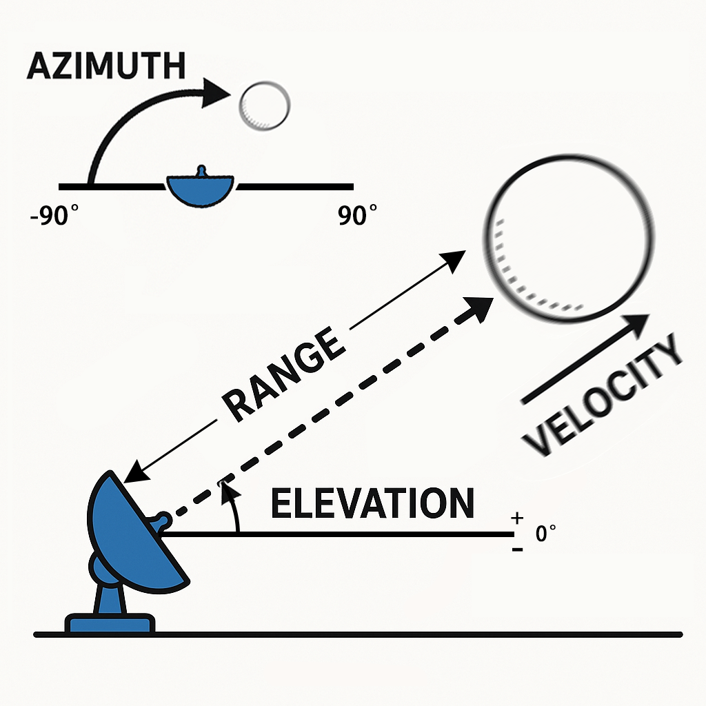
To measure objects surrounding a radar, the following key parameters are used:

• Range: The straight-line distance between the radar and an object.
• Azimuth: The horizontal angle (left to right) between the radar and the object.
• Elevation: The vertical angle (up or down) of the object relative to the radar.
• Velocity: The speed at which the object is moving toward or away from the radar.


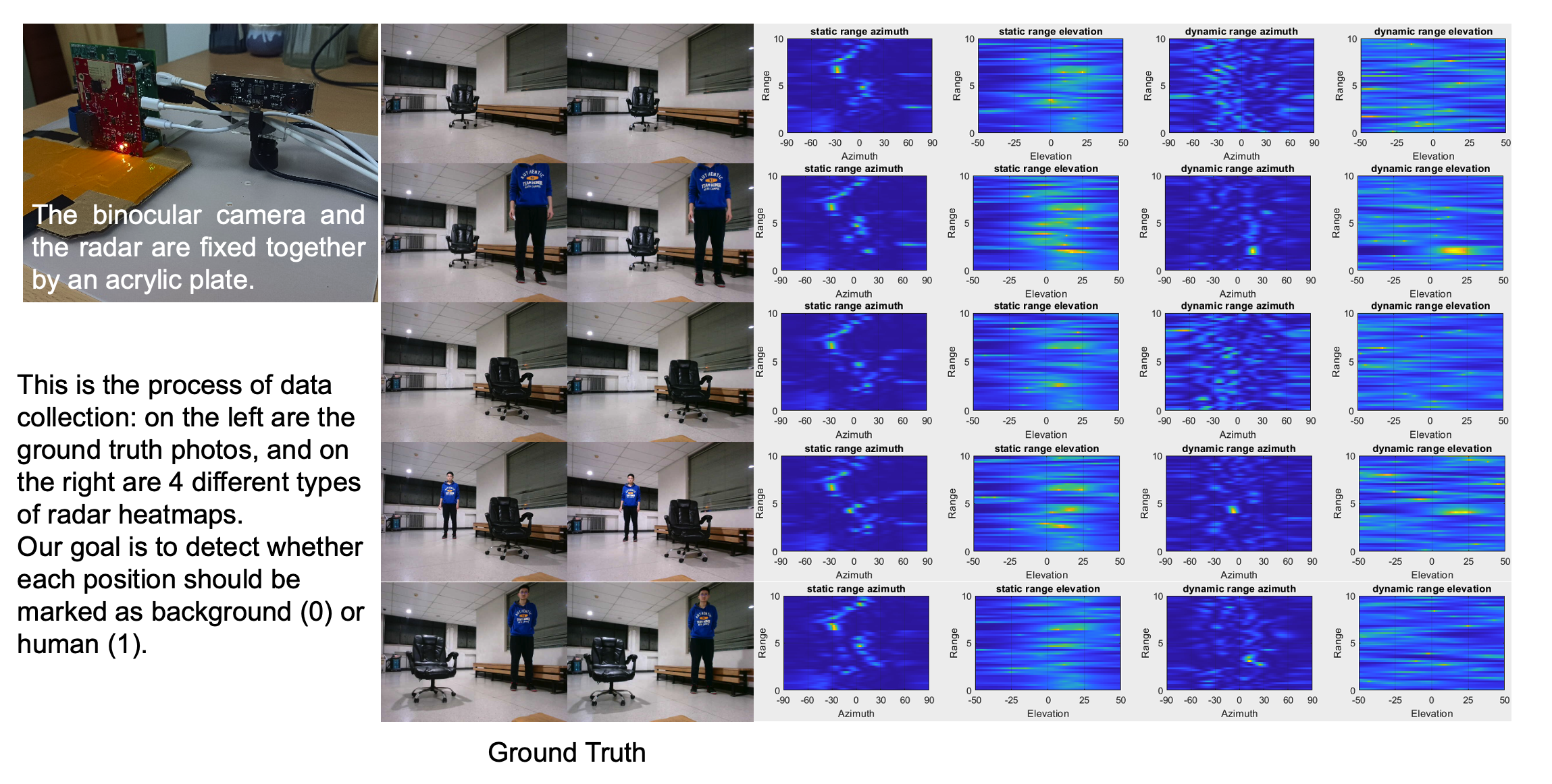
The radar data is processed into multiple heatmaps, each encoding the received signal strength at various positions and directions.

• Static heatmaps emphasize reflections from stationary objects.
• Dynamic heatmaps highlight changes caused by moving objects.

When no object is present at a specific location, the signal consists mostly of background noise and appears weak. In contrast, reflections from an object increase signal intensity, enabling detection of the object.

For example, the static range-azimuth heatmap represents signal strength across different distances (range) and horizontal angles (azimuth), mainly reflected by stationary objects.

Each sample in the dataset is stored in a .mat.pt file as a tensor of shape $7 \times 50 \times 181$, where:

• $7$ is the number of maps (6 heatmaps + 1 semantic label map),
• $50$ represents range bins (distance),
• $181$ represents angular bins, covering angles from $-90^\circ$ to $+90^\circ$ in either the horizontal or vertical plane.

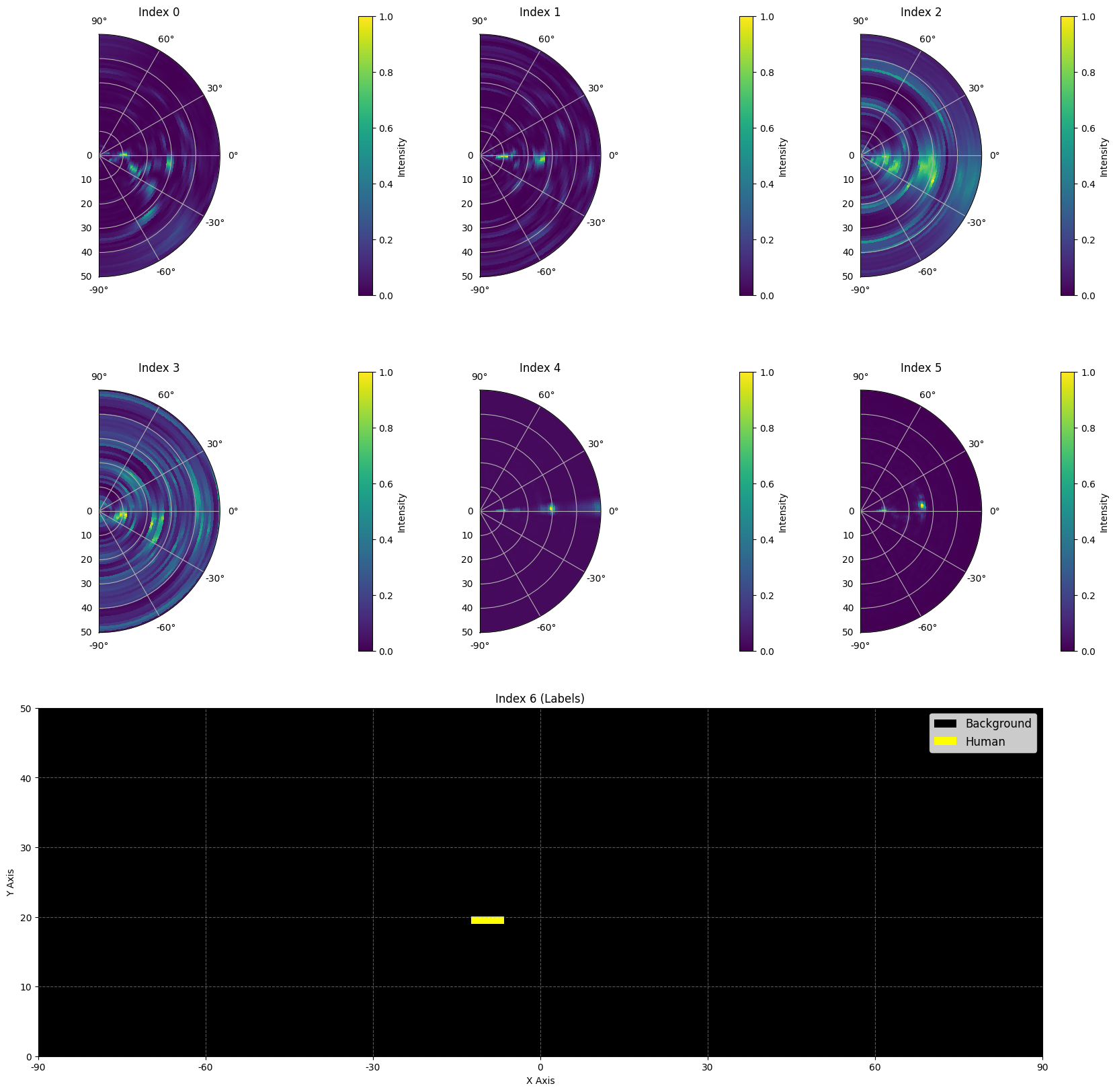
The 6 heatmaps are structured as follows:

• Index 0: Static range-azimuth heatmap
• Index 1: Dynamic range-azimuth heatmap
• Index 2: Static range-elevation heatmap
• Index 3: Dynamic range-elevation heatmap
• Index 4: Static range-velocity heatmap
• Index 5: Dynamic range-velocity heatmap

All values in heatmaps are normalized, so no unit conversion is required.

The map at Index 6 is the semantic label map, stored in range-azimuth format. Each pixel indicates whether a human target is present at that position, using binary values:

• 0: Human absent
• 1: Human present

Here is part of a sample from the dataset:


Task

Your task is to develop a model that takes the first six heatmaps (indices $0$ to $5$) as input, and predicts the semantic label map (index $6$) as the output. The goal is to accurately identify whether a human target is present (1) or absent (0) at each location in the radar’s field of view.

1. Input: A tensor of shape $6 \times 50 \times 181$, representing six radar heatmaps.
2. Output: A tensor of shape $50 \times 181$, representing the target semantic label map.

Accessing Data

You can download the training_set and validation_set through the link below

!pip install gdown

!gdown https://drive.google.com/uc?id=1mXqBIqSfHif3LvJ7Jce1C7addqdfu7B-
!unzip Millimeter-wave_dataset.zip

Dataset Visualization

You can select a piece of data for visualization to understand the specific content represented by each heatmap.

import torch
import matplotlib.pyplot as plt
import numpy as np
import matplotlib
from matplotlib import rcParams
from matplotlib.colors import ListedColormap
from matplotlib.patches import Patch
import matplotlib.gridspec as gridspec

def visualize_pt_file(file_path):
    data = torch.load(file_path)
    print(f"Loaded data shape: {data.shape}")
    num_images = data.shape[0]
    cols = 3
    rows = (num_images + cols - 1) // cols

    fig = plt.figure(figsize=(cols * 5.5, rows * 5.5), constrained_layout=True)

    gs = gridspec.GridSpec(rows, cols, figure=fig)

    colors = ['black', 'yellow']
    cmap_discrete = ListedColormap(colors)

    for i in range(num_images):
        img = data[i].numpy().squeeze()
        img = np.flipud(img)

        if i < 6:
            ax = fig.add_subplot(gs[i // cols, i % cols], projection='polar')
            height, width = img.shape
            angles = np.linspace(-90, 90, width)
            distances = np.linspace(0, 50, height)
            angles_rad = np.radians(angles)
            theta, r = np.meshgrid(angles_rad, distances)
            im = ax.pcolormesh(theta, r, img, shading='auto')

            ax.set_thetalim(np.radians(-90), np.radians(90))
            ax.set_rlim(0, 50)
            ax.set_thetagrids(np.arange(-90, 91, 30))
            ax.set_rticks([0, 10, 20, 30, 40, 50])
            ax.set_rlabel_position(45)
            ax.set_title(f'Index {i}', pad=20)

            plt.colorbar(im, ax=ax, shrink=0.8, label='Intensity')

        else:
            ax = fig.add_subplot(gs[2, :])
            height, width = img.shape
            img_normalized = img + 1
            im = ax.imshow(img_normalized, extent=[-90, 90, 0, height],
                          cmap=cmap_discrete, vmin=0, vmax=4, aspect='auto')

            ax.set_xlabel('X Axis')
            ax.set_ylabel('Y Axis')
            ax.set_title(f'Index {i} (Labels)')

            x_ticks = np.linspace(-90, 90, 7)
            ax.set_xticks(x_ticks)
            ax.set_xticklabels([f'{int(x)}' for x in x_ticks])

            y_ticks = np.linspace(0, height, 6)
            ax.set_yticks(y_ticks)
            ax.set_yticklabels([f'{int(y)}' for y in y_ticks])

            ax.grid(True, linestyle='--', alpha=0.5)

            legend_elements = [
                Patch(facecolor='black', label='Background'),
                Patch(facecolor='yellow', label='Human')
            ]

            ax.legend(handles=legend_elements,
                      loc='best',
                      fontsize='large')

    plt.show()

file_path = f'/content/training_set/1.mat.pt'
visualize_pt_file(file_path)

Loaded data shape: torch.Size([7, 50, 181])


Scoring

The score for this task is based on the accuracy of label recognition. Correctly identifying target points is weighted more heavily than correctly identifying background points.

More specifically:

• Each correctly identified background point earns 1 point.
• Each correctly identified target point earns 1500 points.
• The final score is normalized to a 0-1 scale by comparing it to the maximum possible score.

The following function calculates your score:

import torch
def cal_accuracy(model, test_loader, bonus):
    model.eval()
    total_score = 0
    total_theo = 0

    with torch.no_grad():
        for images, labels, _ in test_loader:
            images = images.cuda() if torch.cuda.is_available() else images
            labels = labels.cuda() if torch.cuda.is_available() else labels

            outputs = model(images)
            outputs = torch.argmax(outputs, dim=1)

            equal_mask = outputs == labels  # correctly predicted masks
            neg_one_mask = labels == 0      # Mask of background categories

            # Calculate the score
            score_neg_one = (equal_mask & neg_one_mask).sum() * 1  # Background category score
            score_other = (equal_mask & ~neg_one_mask).sum() * bonus  # Target category score
            score_theo = neg_one_mask.sum() * 1 + (~neg_one_mask).sum() * bonus  # Full marks in theory

            total_score += score_neg_one + score_other
            total_theo += score_theo

    score = total_score.item() / total_theo.item()
    return score

Example

For a $3\times3$ heatmap, assume the Ground Truth is

$$\begin{bmatrix} 0 & 0 & 0 \\ 1 & 1 & 1 \\ 0 & 0 & 0 \end{bmatrix}$$

The result you identified is

$$\begin{bmatrix} 0 & 1 & 0 \\ 0 & 1 & 0 \\ 0 & 1 & 0 \end{bmatrix}$$

Then there are four correctly identified $0$ and one correctly identified $1$. Your score is $4 + 1500 = 1504$ points. The maximum possible score is $6 + 1500 \times 3 = 4506$, that is, the score for six $0$s and three $1$s. Your normalized score is 1504 / 4506 = 0.33.

$$Score = \frac{4 \times 1 + 1 \times 1500}{6 \times 1 + 3 \times 1500}=0.33$$

import numpy as np
import pandas as pd 
import torch
import torch.nn as nn
import torch.optim as optim
import pickle
import os
import sys
sys.path.append('/bohr/train-4gug/v2')
from dataloader import load_data

class MyModel(nn.Module):
    def __init__(self):
        super(MyModel, self).__init__()
        self.conv1 = nn.Conv2d(in_channels=6, out_channels=16, kernel_size=3, padding=1)  
        self.conv2 = nn.Conv2d(in_channels=16, out_channels=32, kernel_size=3, padding=1)  
        self.conv3 = nn.Conv2d(in_channels=32, out_channels=2, kernel_size=3, padding=1)

        self.relu = nn.ReLU()

    def forward(self, x):
        x = self.relu(self.conv1(x))
        x = self.relu(self.conv2(x))
        x = self.conv3(x)  
        return x

def train(model, train_loader, test_loader, optimizer, criterion, num_epochs=100):
    train_losses = []
    val_losses = []
    
    for epoch in range(num_epochs):
        model.train()
        epoch_loss = 0.0
        batch_count = 0
        
        for images, labels, _ in train_loader:
            images = images.cuda() if torch.cuda.is_available() else images
            labels = labels.cuda() if torch.cuda.is_available() else labels
            
            outputs = model(images)
            outputs = outputs.view(outputs.size(0), outputs.size(1), -1)  # [B, C, H*W]
            labels = labels.view(labels.size(0), -1)  # [B, H*W]
            loss = criterion(outputs, labels)
            
            optimizer.zero_grad()
            loss.backward()
            optimizer.step()
            
            epoch_loss += loss.item()
            batch_count += 1
        
        avg_train_loss = epoch_loss / batch_count
        train_losses.append(avg_train_loss)
        
        model.eval()
        val_loss = 0.0
        val_batch_count = 0
        
        with torch.no_grad():
            for images, labels, _ in test_loader:
                images = images.cuda() if torch.cuda.is_available() else images
                labels = labels.cuda() if torch.cuda.is_available() else labels
                
                outputs = model(images)
                outputs = outputs.view(outputs.size(0), outputs.size(1), -1)
                labels = labels.view(labels.size(0), -1)
                loss = criterion(outputs, labels)
                
                val_loss += loss.item()
                val_batch_count += 1
        
        avg_val_loss = val_loss / val_batch_count
        val_losses.append(avg_val_loss)
        
        if (epoch+1) % 2 == 0:
            print(f'Epoch [{epoch+1}/{num_epochs}], '
                  f'Train Loss: {avg_train_loss:.4f}, '
                  f'Val Loss: {avg_val_loss:.4f}')
    
    return train_losses, val_losses

data_path = '/bohr/train-4gug/v2/training_set'

train_loader, test_loader = load_data(
    base_path=data_path,
    batch_size=4,  
    test_size=0.2
)

model = MyModel()
if torch.cuda.is_available():
    model = model.cuda()

criterion = nn.CrossEntropyLoss()
optimizer = optim.Adam(model.parameters(), lr=0.001) 

train_losses, val_losses = train(
    model=model,
    train_loader=train_loader,
    test_loader=test_loader,
    optimizer=optimizer,
    criterion=criterion,
    num_epochs=40
)

Epoch [2/40], Train Loss: 0.0041, Val Loss: 0.0040
Epoch [4/40], Train Loss: 0.0034, Val Loss: 0.0034

# Please write your model code (including the necessary imported modules, such as torch and torch.nn) below to generate a model structure file that can be easily loaded by the grading platform
model_code = """  
import torch
import torch.nn as nn
class MyModel(nn.Module):
    def __init__(self):
        super(MyModel, self).__init__()
        self.conv1 = nn.Conv2d(in_channels=6, out_channels=16, kernel_size=3, padding=1)
        self.conv2 = nn.Conv2d(in_channels=16, out_channels=32, kernel_size=3, padding=1)
        self.conv3 = nn.Conv2d(in_channels=32, out_channels=2, kernel_size=3, padding=1)  # 5 categories

        self.relu = nn.ReLU()

    def forward(self, x):
        x = self.relu(self.conv1(x))
        x = self.relu(self.conv2(x))
        x = self.conv3(x)  
        return x
"""
# Write code to file
with open('submission_model.py', 'w',encoding="utf-8") as f:
    f.write(model_code)
print("submission_model.py file has been generated.")

# Save the parameters of the model
torch.save(model.state_dict(), 'submission_dic.pth')
print("submission_dic.pth file has been saved.")

submission_dic.pth file has been saved.

# This block mainly specifies the submission format of this question.
import zipfile
import os

# Define the files to zip and the zip file name.
files_to_zip = ['submission_model.py', 'submission_dic.pth']
zip_filename = 'submission.zip'

# Create a zip file
with zipfile.ZipFile(zip_filename, 'w') as zipf:
    for file in files_to_zip:
        # Add the file to the zip fil
        zipf.write(file, os.path.basename(file))

print(f'{zip_filename} Created successfully!')

submission.zip Created successfully!