Stage 1 Test (18 January 2026)

The problem in brief

This is the first-round online test of the Indian National AI Olympiad 2026, sat on 18 January 2026. It has three kinds of items. Section A1 is puzzle-style reasoning: decoding a toy language, choosing which LLM-made features to trust, designing a similarity function, a recursive epidemic, a knight's path. Section A2 contains short modelling puzzles (optimal facility location under two distances, chess match probabilities, reading a price model off a graph, constrained optimisation, Bayes). Section B has four multi-question case studies: a three-class hospital triage classifier, ranking metrics for a retrieval problem, 1-D convolution kernels and pruning a linear classifier. Most answers are an option letter or an integer, usually written as a floor $\lfloor\cdot\rfloor$.

Every numerical answer below was checked by exact or brute-force computation in Python (see the solution code).

How you are scored

Each item is worth the points printed next to it: 3 points for each A1 and A2 item, 1 to 4 points for each case-study question; the total is 70 points. Answers are exact (an option or an integer), so there is no partial credit within a question. No qualifying score is published in the statement.

Answers at a glance

item	answer
A1 Imperial glyphs	樹 造 宮 美 (the options are missing from the published PDF)
A1 Faulty oracle	B: $\{F_1, F_2, F_6\}$
A1 Student search	C
A1 V-67 outbreak	C: 281
A1 Pikachu	E: 25
A2 Godown	11
A2 Blind board gambit	43
A2 Crude curve	92
A2 Catalyst	69
A2 Pit-stop	86
B1 Triage Q1 to Q7	20, 85, C, unchanged, unchanged, option 4 (claims 1, 2, 4), 95
B2 WonkaRank Q1 to Q5	25, option 1, option 6 (none), option 4 (ScoreD only), 27
B3 Convolution Q1 to Q5	A, C, C, B, D
B4 Pruning Q1 to Q3	5, 42, 43

Section A1

Cracking the Imperial Glyphs

Align the sentences that share words. "Apple" appears in sentences 1 to 4 and the glyph pair 蘋果 appears in exactly those, so 蘋果 = apple (two glyphs for one English word). Then 這 appears in "This is..." and "There is...", so it means "this/there is"; 美 = beautiful, 樹 = tree, 宮 = palace, 山 = mountain, 黑 = black, 造 = make, 塗 = paint.

Now the grammar. Two sentences have the same shape as ours:

• "Does the tree make the apple beautiful?" = 樹 造 蘋果 美 ？
• "The mountain paints the palace black." = 山 塗 宮 黑

Both follow subject, verb, object, resulting adjective. A statement drops the question mark. So "The tree makes the palace beautiful" is

$$\text{樹 造 宮 美} .$$

(The answer options are images that did not survive in the published PDF; pick the option that shows exactly these four glyphs in this order. Options with 美 before 宮, or with 這 at the start, are the traps.)

Filtering Fakes with a Faulty Oracle: answer B

Ask, for each feature, whether a small offline model can structurally produce it:

• F1, character count: LLMs read tokens, not characters, so counting characters is a known weakness; a one-line Python len() does it exactly anyway.
• F2, publication year: with no internet and a fixed training cut-off, the model can only guess, and it cannot know events after its cut-off at all.
• F6, named outlet: the model has no source information; it will hallucinate a plausible outlet, and this feature leaks style biases rather than facts.

The others (tone, image-headline match, language, topic, presence of a quote) are judgements about the visible content, which is what such a model does reasonably well. Answer B: $\{F_1, F_2, F_6\}$.

Smart Student Search: answer C

Check each option against the five rules. The Jaro similarity equals 1 exactly when the two strings are identical, and lies in $[0,1]$.

• A gives first and last names equal weight: breaks rule 4.
• B multiplies by $\mathrm{JD}(c, c')$, which is positive for different but similar section codes (9C and 9B): breaks rule 2. It also penalises last names twice as much: breaks rule 4.
• C $= \mathbb 1_{c=c'}\exp\!\big(-2(1-\mathrm{JD}(f,f')) - (1-\mathrm{JD}(l,l'))\big)$: zero when sections differ; the exponent is $\le 0$ so the value is in $(0,1]$; it equals 1 only when both Jaro terms are 1, i.e. both names identical; Jaro is symmetric; the first-name gap is weighted 2, the last-name gap 1. All rules hold.
• D weights the last name twice: breaks rule 4.
• E weights by the lengths of $t$'s names only, so $\mathrm{Sim}(s,t) \ne \mathrm{Sim}(t,s)$ in general: breaks rule 3.
• F can reach 3: breaks rule 5.

Recursive V-67 Outbreak: answer C, 281

Each day: $X_t = 2N_t + 4M_t$; the newcomers add $\frac12 X_t$ normal and $\frac14 X_t$ mutant cases; half of the existing cases recover. So

$$N_{t+1} = \tfrac12 N_t + \tfrac12 X_t, \qquad M_{t+1} = \tfrac12 M_t + \tfrac14 X_t .$$

day	$N_t$	$M_t$	$X_t$	$N_t + M_t$
0	8	8	48	16
1	28	16	120	44
2	74	38	300	112
3	187	94		281

Pikachu's Path to Victory: answer E, 25

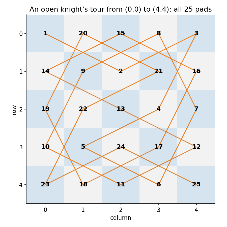
A knight's move changes the colour of the square (on a chessboard colouring), and (0,0) and (4,4) have the same colour, so any path between them visits an odd number of squares. The 5x5 board has 13 squares of the starting colour and 12 of the other, so a path through all 25 squares is not ruled out by parity. A depth-first search finds one: an open knight's tour from corner to opposite corner.

Section A2

The Phulera Godown Showdown: 11

Sachivji (Manhattan). $\sum_i |x - x_i| + |y - y_i|$ separates into an $x$ part and a $y$ part, and each is minimised by a median. With 4 points the median is any value between the 2nd and 3rd order statistics: $x \in [80, 120]$, $y \in [80, 140]$. The rule "take the midpoint of the range" gives $G_S = (100, 110)$.

Pradhanji (generalised KL divergence). $\sum_i x_i \ln\frac{x_i}{u} + (u - x_i)$ is convex in $u$, and its derivative is $-\frac{1}{u}\sum_i x_i + 4$. Setting it to 0 gives $u = \frac14 \sum_i x_i$, the mean. So $G_P = (110, 105)$.

$$D = \sqrt{10^2 + 5^2} = \sqrt{125} \approx 11.18, \qquad \lfloor D \rfloor = 11 .$$

Here is the lesson: absolute error leads to the median, squared error or KL-type divergence to the mean.

The Blind Board Gambit: 43

Anand believes Gukesh plays one of the 5 non-canonical orderings uniformly. For each of his 6 orderings we compute the probability of winning at least 2 of 3 boards, averaged over those 5 orderings. With the Elo formula, the best for Anand is (Y, Z, X), with expected win probability 0.338. Gukesh actually plays (C, A, B):

board	Gukesh	Anand	P(Anand wins)
1	C 1600	Y 1700	0.640
2	A 2000	Z 1500	0.053
3	B 1800	X 1900	0.640

$p = q_1 q_2 q_3 + q_1 q_2 (1-q_3) + q_1 (1-q_2) q_3 + (1-q_1) q_2 q_3 \approx 0.434$, so $\lfloor 100p \rfloor = 43$.

The Crude Curve Forecast: 92

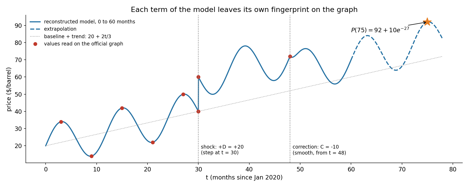
Read each term of the model off its "fingerprint" on the graph:

• Seasonality: peaks at $t = 3, 15, 27$ give period 12, so $\tau_E = 12$; the peaks are where $\sin = 1$.
• Trend and level (before $t = 30$, where only $A + Bt + E\sin$ is active): $P(3) = A + 3B + E = 34$, $P(9) = A + 9B - E = 14$, $P(15) = A + 15B + E = 42$. Subtracting, $12B = 8$, so $B = 2/3$; then $A = 20$ and $E = 12$. Checks: $P(0) = 20$, $P(21) = 22$, $P(27) = 50$, $P(30^-) = 40$, all as drawn.
• Jump at $t = 30$ from 40 to 60: only the Heaviside term $D\,h(t-\tau_D)$ can jump (the $C$ term starts at 0), so $\tau_D = 30$, $D = 20$.
• Smooth bend from $t = 48$: at $t = 48$ the model without $C$ gives $20 + 32 + 20 + 0 = 72$, exactly the marked point, so the $C$ term starts there: $\tau_C = 48$. Afterwards the curve sits lower: without $C$ the value at the trough $t = 57$ would be 66, but the graph shows 56, and at $t = 60$ it would be 80 but the graph ends at 70. So $C = -10$ (the factor $1 - e^{-9}$ is 1 for practical purposes).

Then

$$P(75) = 20 + \tfrac23\cdot 75 + 20 - 10\,(1 - e^{-27}) + 12\sin\!\big(\tfrac{2\pi\cdot 75}{12}\big) = 20 + 50 + 20 - 10 + 12 + 10e^{-27},$$

since $75/12 = 6.25$ puts the sine at a peak. So $P(75)$ is a hair above 92 and $\lfloor P(75) \rfloor = 92$.

The Catalyst Constraint: 69

Maximise $16c_A - 2c_A^2 + 24c_B - 3c_B^2$ with $c_A + c_B \le 5$, $c_A, c_B \ge 0$. Unconstrained, each pathway peaks at $c_A = 16/4 = 4$ and $c_B = 24/6 = 4$, which would need 8 moles of catalyst. So the constraint binds and the marginal yields must be equal:

$$16 - 4c_A = 24 - 6c_B, \quad c_A + c_B = 5 \;\Rightarrow\; c_B = 2.8,\; c_A = 2.2 .$$

$d_A = 35.2 - 9.68 = 25.52$, $d_B = 67.2 - 23.52 = 43.68$, total $69.2$, so the answer is 69. (Equal marginal returns at the optimum is the same idea as a Lagrange multiplier, or as a learning-rate budget split between two objectives.)

The Pit-Stop Paradox: 86

Each (weather, strategy) pair gets probability $P(\text{weather})\,P(\text{strategy}\mid\text{weather})\,P(H\mid\text{strategy},\text{weather})$:

	neither	only V	only H	both
no rain (x 0.5)	0.05625	0.12	0.005	0.04125
rain (x 0.5)	0.0125	0.0025	0.0475	0.225

$P(H \text{ wins}) = 0.51$, of which "neither pitted" accounts for $0.06875$. Hence

$$P(\text{at least one pitted} \mid H) = 1 - \frac{0.06875}{0.51} \approx 0.865, \qquad \lfloor 86.5 \rfloor = 86 .$$

Section B1: Triage classifier

First rebuild the full confusion matrix of the 1000 test patients (600 / 300 / 100 per class). Sensitivities give the diagonal (510, 210, 80); the two "egregious error" rates give $1 \to 3$: $0.0333 \times 600 = 20$ and $3 \to 1$: $0.10 \times 100 = 10$. Then each row sums to its class size, so $1 \to 2$ is 70 and $3 \to 2$ is 10. The last unknown is how class 2's 90 errors split between classes 1 and 3. Specificity of class 1 decides it: 10 % of the 400 non-class-1 patients, i.e. 40, are predicted class 1, of which 10 come from class 3, so $2 \to 1$ is 30 and $2 \to 3$ is 60.

actual \ predicted	1	2	3
1 (600)	510	70	20
2 (300)	30	210	60
3 (100)	10	10	80

Check: this matrix gives specificities 0.900, 0.886 and 0.911, matching the stated 0.90, 0.89 and 0.91.

• Q1: 20. Missed ICU patients are $1 - \text{sensitivity}_3 = 20\%$.
• Q2: 85. This is just the sensitivity of class 1.
• Q3: C. Expected ICU flags per day $= 200\,(0.10\,\text{TPR} + 0.90\,\text{FPR})$: A 15.6, B 21.6, C 24.6, D 31.2. C is the most sensitive point that stays under 25 beds.
• Q4: the curve is unchanged. A ROC curve only depends on the ranking of the scores. A strictly increasing transformation keeps every ranking, so each threshold $t$ has an equivalent threshold $t^{1.5}$ with the same TPR and FPR. (Strictly, $s^{1.5}$ is only a real, increasing function for $s \ge 0$; the statement calls it monotonic, which is what matters.)
• Q5: the curve is unchanged. TPR and FPR are computed within each class, so changing the class proportions does not move the curve (as long as the score distributions within each class stay the same). What changes is precision and the number of flagged patients: at 25 % prevalence the bed constraint of Q3 would select a different point.
• Q6: option 4 (claims 1, 2 and 4). Claim 1 holds: two independent binary classifiers can contradict each other ("not class 1" by the first and "not class 3" by the second is consistent, but "class 1" by the first and "class 3" by the second is not), and pairwise votes can form cycles. Claim 2 holds: the domain analysis says the two boundaries depend on different criteria, which a single score with two thresholds (parallel boundaries) cannot represent, but Y can. Claim 3 is false: Z throws away the ordering, trains each classifier on only part of the limited data, and its 1-vs-3 classifier adds little. Claim 4 holds: squared loss on ordinal targets acts as regression, which respects the order 1 < 2 < 3, while hinge loss only cares about the margin; but squared loss also punishes points that are far on the correct side and is dominated by outliers. Claim 5 is false: squared loss grows quadratically with the error, so it is less robust to outliers than logistic loss, which grows only linearly.
• Q7: 95. Multiply the confusion matrix by the benefit matrix cell by cell: $510\cdot100 + 70\cdot50 + 210\cdot100 + 60\cdot50 + 10\cdot50 + 80\cdot200 = 95\,000$, i.e. 95 points per patient.

Section B2: WonkaRank

There are $R = 4$ relevant chocolates: D1 (10), D5 (3), D8 (5), D9 (3).

• Q1: 25. The top 5 bought are D2, D3, D5, D6, D7: only D5 is relevant, so recall is $1/4$.
• Q2: option 1. Strategy A gives a positive score only to D1, D2, D5, D8, so it effectively retrieves 4 chocolates, 3 of them relevant: precision 0.75, recall 0.75. Strategy B also gives score 1 to D3, D4, D7, D9, so it retrieves 8 chocolates (D6 alone scores 0), now including D9: recall 1, precision 4/8 = 0.5. B improves recall but reduces precision.
• Q3: option 6, none of the above. Compute rather than guess. $\mathrm{DCG}_A = \frac{3}{1} + \frac{10}{\log_2 3} + \frac{5}{2} = 11.81$ and $\mathrm{DCG}_B = \frac{5}{1} + \frac{3}{\log_2 3} + \frac{10}{2} = 11.89$. B wins narrowly, yet B places the most relevant chocolate (D1) later than A does (rank 3 against rank 2). So the explanation cannot be "DCG puts the highest-relevance item first" (option 2). DCG simply adds discounted gains, and B's gain from putting 5 at rank 1 and 3 at rank 2 slightly outweighs A's. The other options are false outright: order matters, gains are graded, all ranks count, irrelevant items contribute 0. (Option 2 may be the intended answer, but the numbers contradict it.)
• Q4: option 4, ScoreD only. Scores of the top documents: ScoreA puts D2 and D5 first (7 each), giving precision 1/2. ScoreB counts the ingredients present: D2 and D5 again (3 each), precision 1/2. ScoreC ties D1, D2, D5, D8 at 4, and the ID tie-break keeps D1, D2, precision 1/2. ScoreD $= \frac{\sum d_i w_i}{1 + \sum d_i}$ rewards concentration on the heavy ingredients and puts D1 and D8 (score 2) first: precision 1. Normalising by the number of ingredients penalises chocolates that are merely "large", such as D2 with caramel added.
• Q5: 27. ScoreA ranking: D2, D5, D1, D8, D3, ... The relevant chocolates in the top 5 are at ranks 2, 3, 4, with inspection probabilities 0.5, 0.3, 0.3. PI-Recall@5 $= (0.5 + 0.3 + 0.3)/4 = 0.275$.

Section B3: Convolution kernels

The definition $y_i = \sum_j h_j x_{i+k-j}$ is a true convolution: the kernel is reversed before sliding. A useful trick: the sum $S = \sum_i y_i$ of a zero-sum kernel telescopes and only depends on a few values at the ends of the signal.

• Q1: A, [8, 5, 11]. The padded signal is $[3, 2, 1, 3, 4, 3]$ and the reversed kernel is $[2, 1]$. With stride 2 the windows are $(3,2), (1,3), (4,3)$: $6+2 = 8$, $2+3 = 5$, $8+3 = 11$.
• Q2: C, [1, -2, 1]. A constant signal must give $S = 0$, so the kernel must sum to 0, which leaves B, C, D and F. For $[1,-2,1]$, $S = x_1 - x_2 - x_{n-1} + x_n$: it is 0 for the smooth $x$ and $-10$ for the fluctuating $z$. Each first-difference kernel instead gives $|S|$ larger for $x$ than for $z$ or about equal ($[-1,0,1]$: $-12$ vs $-6$; $[-1,1,0]$: $-6$ vs $2$; $[1,0,-1]$: $12$ vs $6$). A second difference measures curvature, i.e. changes of direction.
• Q3: C, [1, -2, 1]. The discrete second derivative $x_i - 2x_{i+1} + x_{i+2}$ is 0 at constant velocity. For the accelerating $x$ it gives $1, 1, 1$ ($S = 3 > 0$), for the decelerating $w$ it gives $-1, -1, -1$ ($S = -3$).
• Q4: B, [-1, 2, -1]. This is minus the second difference, so it is 0 on any straight line (constant or linear), and therefore 0 for the smooth $z$. On $x$ it gives $-4, 10, -4, -2$, so $S_{\text{abs}} = 20$, with the big response centred on the spike. Using $S_{\text{abs}}$ rather than $S$ matters: the plain sum would telescope back to a few end values.
• Q5: D, [1, -1, 1, -1]. A length-4 kernel on a length-4 signal gives a single output $y = h_1x_4 + h_2x_3 + h_3x_2 + h_4x_1$. For it to vanish on every symmetric signal ($x_1 = x_4$, $x_2 = x_3$) we need $h_4 = -h_1$ and $h_3 = -h_2$; only D satisfies this. It gives $y = 0$ on $[2,5,5,2]$ and $y = -3 \ne 0$ on $z$. Caveat: no single linear output can be nonzero on every asymmetric signal (D also gives 0 on $[1,1,2,2]$), because the asymmetric part of a length-4 signal has two degrees of freedom; detecting all of them would need two outputs.

Section B4: Pruning a linear classifier

• Q1: 5. The first four rows of $X$ are the identity, so $s_1, \dots, s_4$ are $w_1, \dots, w_4$; then $s_5 = w_1 + w_2$ and $s_6 = w_1 + w_3 + w_4$. Option A: $w_1 = 2$, $w_3 = 1$, $w_4 = -1$ and $w_2 = s_5 - w_1 = -1$, so $s = (2, -1, 1, -1, 1, 2)$: every sign matches $y$, accuracy 100 %. Option B: $w_1 = 3$, $w_2 = -5$, $w_4 = -1$ and $w_3 = 1 - 3 + 1 = -1$, so $s_3 = -1$ and $s_5 = -2$: two wrong signs, accuracy 4/6. Choose A: $\lVert w\rVert_1 = 2 + 1 + 1 + 1 = 5$.
• Q2: 42. Unpruned, every example is correctly classified (scores $1,1,1,1,1,1,0$, with 0 counting as class 0). Feature 7 already has weight 0, so pruning it costs nothing; every other feature carries a whole example. Removing feature $j \le 5$ sets that example's score to 0, so it flips to class 0, a mistake, and also shifts the last example's score to $+1$, a second mistake. Removing feature 6 only costs example 6. So the best pair is $\{6, 7\}$ with accuracy 6/7, and $6 \cdot 7 = 42$. (Exhaustive search over the 21 pairs confirms it is the unique best.)
• Q3: 43. After pruning, the scores are $(1,1,1,1,1,0,-5)$. Any bias $b \ge 1$ makes example 6 positive while example 7 stays negative ($-5 + 3 < 0$): accuracy 100 %. Negative biases push the five ones to $\le 0$. The smallest $|b|$ with full accuracy is $b^\ast = 1$, so the answer is $42 + 1 = 43$. (The mean-preserving correction of the background section agrees: the removed contribution is $(0,0,0,0,0,1,5)$, so $\mu_S = 6/7 \approx 0.86$, which also restores 100 % accuracy.)

What to remember

• Turn every metric question into a confusion matrix. Sensitivities, specificities and error rates are just row and column sums; once the matrix is rebuilt, benefits, capacities and precision all follow by arithmetic.
• ROC curves only see rankings within each class. Monotone transforms of the score and changes in class prevalence leave them unchanged. Prevalence still matters for precision, for the number flagged and for choosing the operating point.
• The loss decides the optimal summary. Absolute error gives the median, squared error and KL-type divergence give the mean, and equal marginal returns at the optimum is the Lagrange condition.
• Compute, then match the option. On DCG the intuitive choice ("highest relevance first") is contradicted by the numbers. Small brute-force scripts (DFS for the knight, enumeration for the pruning pairs) settle what intuition cannot.
• Kernels are finite-difference operators. $[1,-1]$ measures slope, $[1,-2,1]$ curvature or acceleration, $[-1,2,-1]$ spikes. Zero-sum kernels ignore constants, and sums of their outputs telescope.