Indonesia IOAI selection 2026 · Correction by IOAI Training

Hybrid Riverflow

This page gives the full approach. Read it once you have searched.

Metric: MAE
Evaluated on: held-out validation (official test labels are private)
Our score: MAE 1.33 (5-fold CV), 1.40 on split42
Expected level: starter ETS baseline: MAE 4.756 on split42

Expected level reached

We solved the problem ourselves: downloaded the data, ran the experiments and measured the score below. The statement and data belong to their organisers.

The problem in brief

Each sample is a synthetic record of daily river discharge at one site, between 50 and 60 days long. You must predict a single number: the average discharge over the next 12 days. There are 1200 training series with their answer and 400 test series. The series do not all behave alike: some climb steadily, some oscillate, some wander around a level and occasionally jump. The organisers warn that treating every series as following one pattern will not be optimal, hence the name "hybrid".

The competition ran on Kaggle, whose test labels are private (and need a login). We use the public data bundle from the organisers' Google Drive and evaluate on the training data: the starter notebook's own 80/20 split (random_state=42), so we can compare with its baseline, plus 5-fold cross-validation on all 1200 series. All scores here are on held-out training data, not on the official test set.

How you are scored

Mean absolute error between the predicted and the true 12-day means:

\text{MAE} = \frac{1}{n}\sum_{i=1}^{n} \lvert \hat y_i - y_i \rvert, \qquad y_i = \frac{1}{12}\sum_{t=T_i+1}^{T_i+12} x_{i,t}.

Lower is better. The Kaggle leaderboard is not public, so the only published reference is the starter notebook's baseline, a damped Holt-Winters model fitted to each series, which scores 4.756 on that 80/20 split. We reran it and got exactly the same number.

First look at the data

Plot a few dozen series and four families appear at once (the data's metadata.json confirms there are 4 hidden regimes):

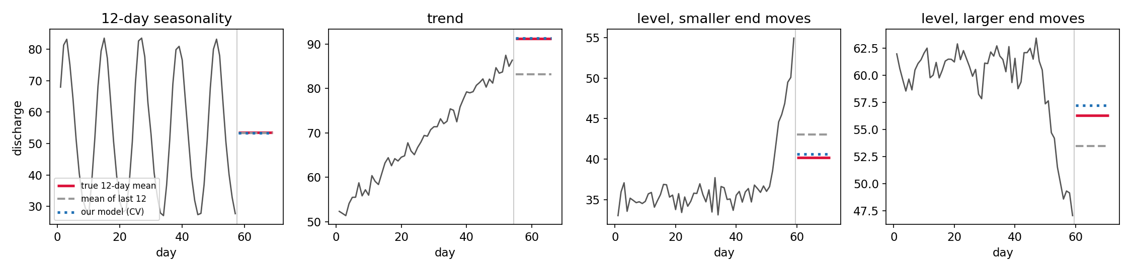
One example per regime, with the true 12-day mean, the naive forecast and our model

12-day seasonality: a clean oscillation with period 12.
Trend: a steady climb (or fall) with a little noise.
Level series that wander around a constant, sometimes with a sudden move near the end: a spike, a drop, a burst. The future mean usually falls back towards the old level, but not all the way.

Two quick checks set the scale of the problem: predicting the overall mean of all targets gives MAE 14.8; predicting the mean of the last 12 days gives 3.93, already better than the official baseline.

A first baseline

Why does the starter's Holt-Winters model (4.756) lose even to "the mean of the last 12 days" (3.93)? Because it is a local model: it is fitted on the 50 to 60 points of a single series, with smoothing, trend, damping and 12 seasonal coefficients to estimate. That is a lot of parameters for 55 noisy points, and on the level series it happily extrapolates a short-lived jump as if it were a trend.

Each simple rule is good on one regime and bad on another (see the figure in the next section):

the mean of the last 12 days is nearly perfect on seasonal series but misses trends by half a cycle's worth of growth;
a linear extrapolation to day $T+6.5$ (the centre of the forecast window) is good on trends (MAE 2.67 overall) but bad on level series, where it extends a final jump.

The key idea

Learn one global model from all 1200 series, on features that make the regimes easy to tell apart, and predict a correction to a simple forecast.

Three ingredients make this work.

1. Why the mean of the last 12 days is the right anchor. For a series that is periodic with period 12, any 12 consecutive days cover each phase exactly once, so

\frac{1}{12}\sum_{t=T-11}^{T} x_t \;=\; \frac{1}{12}\sum_{t=T+1}^{T+12} x_t

up to noise: the seasonal part cancels. For the other regimes it is a sensible level estimate too. So we define $m_{12}$ as that mean and train the model to predict $y - m_{12}$ , and we express every level feature relative to $m_{12}$ as well. A river at 30 and a river at 90 with the same shape then look identical to the model: the problem becomes scale-free, and 1200 series share what they teach.

2. Features that reveal the regime. A tree model can only use the regime if it can see it:

autocorrelations at lags 1, 6 and 12 (seasonal series have $\rho_6 \approx -0.8$ and $\rho_{12} \approx +0.8$ );
the slope of a fitted line, its extrapolation at $T+6.5$ , and the residual spread around it (trends are almost perfectly linear);
the level of the series before the last 12 days (where a level series will return to), its minimum and maximum, and the last 24 values right-aligned (the shape of the final move);
two small model-based forecasts: an AR(1) process $x_{t+1}-\mu = \varphi(x_t-\mu)$ fitted to the series, whose 12-day mean forecast is $\mu + (x_T-\mu)\,\frac{1}{12}\sum_{h=1}^{12}\varphi^h$ , and the same after removing the period-12 profile.

3. Global beats local. A local model has 55 points to learn from. A global model has $1200 \times 55$ , and it learns things no single series can tell it, for example how much of a final jump typically survives over the next 12 days. That is exactly the hard part of the level regime.

The organisers' configuration hints that they intended to first cluster the series into 4 groups, then fit one model per cluster. We tried it, and it did not help: with good features, the trees already split by regime on their own, and separate models only see a quarter of the data each.

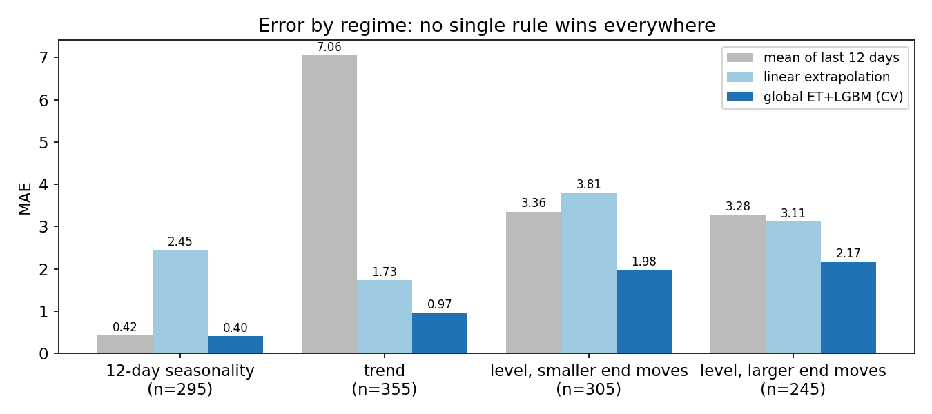
MAE by regime for the two simple rules and our model

The regimes here come from k-means on a few shape statistics, only for this diagnosis. The global model is never worse than the best simple rule in any regime, and much better on trends and level series. The errors that remain (about 2 on level series) are mostly irreducible: nobody can predict the noise of the next 12 days.

The full solution

For each series keep its first $T$ values (the NaNs after $T$ only mark a shorter series).
Compute about 50 features: $T$ , slopes, autocorrelations, spread, levels relative to $m_{12}$ , the last 24 values relative to $m_{12}$ , the AR(1) forecasts.
Target: $r = y - m_{12}$ .
Fit an ExtraTrees regressor (500 trees, min_samples_leaf=2, max_features=0.5) and a LightGBM model with an L1 objective (the metric is MAE, so we fit the median, not the mean). Average their two predictions of $r$ .
Predict $\hat y = m_{12} + \hat r$ .

r = y_train - F_train.m12
preds = [m.fit(F_train, r).predict(F_test) for m in (extra_trees, lgbm_l1)]
y_hat = F_test.m12 + np.mean(preds, axis=0)

Everything trains in a few seconds on a CPU.

Results

approach	split42 val. MAE	5-fold CV MAE (no-fit rules: all 1200 series)
mean of all training targets		14.80
last observed value		7.24
local damped Holt-Winters (starter baseline)	4.756
mean of the last 12 days	3.932
linear extrapolation to day $T+6.5$	2.668
global ridge regression on our features	1.685	1.631
global LightGBM (L1)	1.446	1.373
global ExtraTrees	1.436	1.360
ExtraTrees + k-means cluster id as a feature		1.365
one ExtraTrees per k-means cluster (the "intended" hybrid)		1.382
ExtraTrees + AR(1) forecast features		1.334
ExtraTrees + LightGBM average, all features (final)	1.395	1.331

On the starter notebook's own split, our model cuts the official baseline's error by more than a factor of 3 (4.756 to 1.395). The 5-fold CV figure, 1.33, is the more reliable estimate of what to expect on the private test set.

What to remember

Global models beat local ones when you have many short series: one model trained on all of them learns the patterns that no single 55-point series can reveal.
Make the problem scale-free: predict a correction to a strong simple forecast ( $y - m_{12}$ ) and express features relative to the recent level.
Know your simple forecasts and when each one is right: the mean over a full period cancels seasonality, a line handles trends. They make excellent features.
Explicit clustering is not needed when the features expose the regimes: trees split on them by themselves, and per-cluster models waste data.
Match the loss to the metric: for MAE, an L1 objective (the conditional median) is the natural choice.

Full code (solution.py)

"""Hybrid Riverflow (Pelatnas 1 IOAI 2026, Indonesia, simulation 2) -- worked solution.

Each row is one synthetic daily river-discharge series of length T in [50, 60] (x_1..x_60, NaN
after T). Target: mean of the next 12 days. Metric: MAE. Test labels are private (Kaggle), so we
evaluate on the training data: the starter notebook's 80/20 split (random_state=42) and 5-fold CV.

Data: Drive zip 180yS7AFlg8YXv0edEoDOg_EZxxes05EK (train.csv, test.csv, sample_submission.csv)
  curl -L -o d.zip 'https://drive.usercontent.google.com/download?id=180yS7AFlg8YXv0edEoDOg_EZxxes05EK&export=download'

Idea: ONE global model learns from all 1200 series at once (a local model sees 50 points, a global
one sees 1200 x 50), on hand-made, scale-free features: everything is expressed relative to the
mean of the last 12 days, which is also the base forecast; the model predicts the correction.
The four hidden regimes (trend, 12-day seasonality, mean reversion, end-of-series shock) are
separated by the trees themselves through autocorrelation / slope features.

Run: python solution.py DATA_DIR [--ets] [--figures]
"""
import sys, warnings
import numpy as np
import pandas as pd
import lightgbm as lgb
from sklearn.ensemble import ExtraTreesRegressor
from sklearn.model_selection import KFold, train_test_split

warnings.filterwarnings("ignore")
args = [a for a in sys.argv[1:] if not a.startswith("--")]
DATA_DIR = args[0] if args else "work"
H = 12


# ---------------------------------------------------------------------------------------------
# Features
# ---------------------------------------------------------------------------------------------
def get_series(df):
    X = df[[f"x_{i}" for i in range(1, 61)]].values
    return [X[i, :L] for i, L in enumerate(df.obs_len.values)]


def linear_forecast(s):
    """Fit a line, return its mean value over the next 12 days (= value at T + 6.5) and the slope."""
    t = np.arange(len(s))
    b, a = np.polyfit(t, s, 1)
    return a + b * (len(s) - 1 + (H + 1) / 2), b


def acf(s, lag):
    s = s - s.mean()
    return (s[lag:] * s[:-lag]).sum() / (s * s).sum()


def ar1_forecast(s):
    """AR(1) around a mean: x_{t+1} - mu = phi (x_t - mu); mean of the 12 forecasts."""
    phi, c = np.polyfit(s[:-1], s[1:], 1)
    phi = np.clip(phi, -0.99, 0.99)
    mu = c / (1 - phi)
    return mu + (s[-1] - mu) * np.mean(phi ** np.arange(1, H + 1)), phi


def seasonal_ar_forecast(s):
    """Remove the period-12 profile, AR(1) on the rest, add the profile back (its mean over a full
    period is 0, so the 12-day mean only needs the deseasonalised forecast)."""
    ph = np.arange(len(s)) % 12
    prof = np.array([s[ph == k].mean() for k in range(12)]) - s.mean()
    return ar1_forecast(s - prof[ph])[0]


def features(s):
    T, m12 = len(s), s[-12:].mean()
    lin, slope = linear_forecast(s)
    lin24, slope24 = linear_forecast(s[-24:])
    t = np.arange(T)
    resid = s - np.polyval(np.polyfit(t, s, 1), t)
    ar, phi = ar1_forecast(s)
    ar30, _ = ar1_forecast(s[-30:])
    f = dict(T=T, m12=m12, slope=slope, slope24=slope24, std=s.std(), resid_std=resid.std(),
             acf1=acf(s, 1), acf6=acf(s, 6), acf12=acf(s, 12), phi=phi)
    # levels, all relative to the recent mean m12 (scale-free)
    levels = dict(m_all=s.mean(), m_first=s[:-12].mean(), med_first=np.median(s[:-12]), last=s[-1],
                  m3=s[-3:].mean(), m6=s[-6:].mean(), lin=lin, lin24=lin24, mn=s.min(), mx=s.max(),
                  ar=ar, ar30=ar30, sar=seasonal_ar_forecast(s))
    f.update({k + "_r": v - m12 for k, v in levels.items()})
    for j in range(1, 25):                                  # the last 24 days, right-aligned
        f[f"lag{j}_r"] = s[-j] - m12
    return f


def build(df):
    return pd.DataFrame([features(s) for s in get_series(df)])


# ---------------------------------------------------------------------------------------------
# Model: average of ExtraTrees and LightGBM (L1 objective), predicting y - m12
# ---------------------------------------------------------------------------------------------
def make_models():
    return [ExtraTreesRegressor(500, min_samples_leaf=2, max_features=0.5, n_jobs=2, random_state=0),
            lgb.LGBMRegressor(n_estimators=600, learning_rate=0.03, num_leaves=15, min_child_samples=10,
                              subsample=0.8, subsample_freq=1, colsample_bytree=0.7, objective="l1",
                              num_threads=2, verbose=-1, random_state=0)]


def fit_predict(Ftr, ytr, Fte):
    r = ytr - Ftr.m12.values
    preds = [m.fit(Ftr.values, r).predict(Fte.values) for m in make_models()]
    return Fte.m12.values + np.mean(preds, axis=0)


def mae(a, b):
    return float(np.mean(np.abs(np.asarray(a) - np.asarray(b))))


def ets_forecast(s):
    """The organisers' baseline: damped Holt-Winters per series, fallback damped Holt."""
    from statsmodels.tsa.holtwinters import ExponentialSmoothing
    for kw in (dict(seasonal="add", seasonal_periods=12), dict(seasonal=None)):
        try:
            fit = ExponentialSmoothing(s, trend="add", damped_trend=True, initialization_method="estimated",
                                       **kw).fit(optimized=True, use_brute=True)
            return float(np.mean(fit.forecast(H)))
        except Exception:
            pass
    return float(np.mean(s[-H:]))


def main():
    train = pd.read_csv(f"{DATA_DIR}/train.csv")
    test = pd.read_csv(f"{DATA_DIR}/test.csv")
    F, Ft, y = build(train), build(test), train.target.values

    # 1) the starter notebook's split, to compare with its ETS baseline
    tr, va = train_test_split(np.arange(len(train)), test_size=0.2, random_state=42)
    print("split42 validation MAE")
    print(f"  mean of last 12 days     {mae(F.m12.values[va], y[va]):.3f}")
    print(f"  linear extrapolation     {mae(F.m12.values[va] + F.lin_r.values[va], y[va]):.3f}")
    if "--ets" in sys.argv:
        S = get_series(train)
        print(f"  local ETS (starter)      {mae([ets_forecast(S[i]) for i in va], y[va]):.3f}")
    print(f"  global ET+LGBM (ours)    {mae(fit_predict(F.iloc[tr], y[tr], F.iloc[va]), y[va]):.3f}")

    # 2) 5-fold CV on all 1200 series
    oof = np.zeros(len(y))
    for a, b in KFold(5, shuffle=True, random_state=0).split(F):
        oof[b] = fit_predict(F.iloc[a], y[a], F.iloc[b])
    print(f"5-fold CV MAE, global ET+LGBM: {mae(oof, y):.3f}")

    # 3) final model on all training data -> submission
    sub = pd.DataFrame({"id": test.id, "target": fit_predict(F, y, Ft)})
    sub.to_csv("submission.csv", index=False)
    print("wrote submission.csv", sub.shape)

    if "--figures" in sys.argv:
        figures(train, F, y, oof)


def figures(train, F, y, oof):
    import matplotlib
    matplotlib.use("Agg")
    import matplotlib.pyplot as plt
    from sklearn.cluster import KMeans
    from sklearn.preprocessing import StandardScaler
    plt.rcParams.update({"font.size": 11})
    # regimes recovered by k-means on a few shape statistics (for the explanation only)
    Z = np.c_[F.acf1, F.acf6, F.acf12, np.abs(F.slope) * F["T"] / F["std"], F.resid_std / F["std"],
              F.last_r / F["std"]]
    lab = KMeans(4, n_init=20, random_state=2026).fit_predict(StandardScaler().fit_transform(Z))
    order = [int(np.argmax([F.acf12[lab == k].mean() for k in range(4)])),      # seasonal
             int(np.argmax([F.slope[lab == k].mean() for k in range(4)]))]      # trend
    rest = [k for k in range(4) if k not in order]
    rest.sort(key=lambda k: np.abs(F.last_r[lab == k]).mean())                   # calm, then shock
    order += rest
    names = ["12-day seasonality", "trend", "level, smaller end moves", "level, larger end moves"]
    S = get_series(train)
    fig, axes = plt.subplots(1, 4, figsize=(15, 3.6))
    for ax, k, nm in zip(axes, order, names):
        i = np.where(lab == k)[0][3]
        s = S[i]; T = len(s)
        ax.plot(np.arange(1, T + 1), s, color="#555", lw=1.3)
        ax.hlines(y[i], T + 1, T + 12, color="crimson", lw=2.5, label="true 12-day mean")
        ax.hlines(F.m12[i], T + 1, T + 12, color="#999", ls="--", lw=2, label="mean of last 12")
        ax.hlines(oof[i], T + 1, T + 12, color="#2171b5", ls=":", lw=2.5, label="our model (CV)")
        ax.axvline(T + 0.5, color="#ccc", lw=1)
        ax.set_title(nm); ax.set_xlabel("day")
    axes[0].set_ylabel("discharge"); axes[0].legend(fontsize=8, loc="lower left")
    fig.tight_layout(); fig.savefig("figures/regimes.png", dpi=150, facecolor="white"); plt.close(fig)

    fig, ax = plt.subplots(figsize=(9, 4))
    x = np.arange(4); w = 0.27
    for j, (pred, nm, col) in enumerate([(F.m12.values, "mean of last 12 days", "#bbbbbb"),
                                         (F.m12.values + F.lin_r.values, "linear extrapolation", "#9ecae1"),
                                         (oof, "global ET+LGBM (CV)", "#2171b5")]):
        v = [mae(pred[lab == k], y[lab == k]) for k in order]
        ax.bar(x + (j - 1) * w, v, w, label=nm, color=col)
        for xi, vi in zip(x, v):
            ax.text(xi + (j - 1) * w, vi + 0.1, f"{vi:.2f}", ha="center", fontsize=8)
    ax.set_xticks(x); ax.set_xticklabels([f"{n}\n(n={np.sum(lab == k)})" for n, k in zip(names, order)])
    ax.set_ylabel("MAE"); ax.set_title("Error by regime: no single rule wins everywhere"); ax.legend(fontsize=9)
    fig.tight_layout(); fig.savefig("figures/mae_by_regime.png", dpi=150, facecolor="white"); plt.close(fig)


if __name__ == "__main__":
    main()