Monte Carlo Simulation

The problem in brief

The notebook first shows a worked example: throw a fair die until an even number appears. The expected number of throws, 2, is computed analytically and then estimated by simulating the experiment many times and averaging. You then write two Monte Carlo programs of your own. Soal A: keep throwing until the running total of the faces reaches at least 12; how many throws does that take on average? Soal B: throw until the first 6; given that this happened on exactly the 5th throw, how many odd faces do you expect to have seen? It is an exercise from the exhibition final of the Indonesian national science olympiad (OSN) in AI.

How you are scored

Soal A is worth 30 points and Soal B 70 points. The deliverable is a working simulation whose estimate is close to the true expectation. We therefore give, for each question, a Monte Carlo estimate with its uncertainty and check it against the exact value derived by hand.

One remark on the worked example: it writes $\mathbf E[X] = \frac{1}{1-p}$ for the geometric distribution. The correct formula is $\mathbf E[X] = \frac1p$. With $p = 0.5$ both give 2, which hides the slip, but with $p = 1/6$ (waiting for a 6) the answer is 6, not 1.2.

The key idea

A Monte Carlo estimate is just a sample mean of independent runs of the experiment, so it comes with a standard error: if the runs have standard deviation $\sigma$, the mean of $N$ runs has error about $\sigma/\sqrt N$. This tells you how many runs you need and whether your simulation agrees with a formula.

The two questions test two different skills:

• A is about simulating a stopping rule correctly: stop as soon as the total reaches 12, and count the throw that crossed the threshold.
• B is about simulating a conditional expectation. There are two honest ways to do it. You can simulate the unconditional experiment and keep only the runs that satisfy the condition (rejection sampling). Or you can work out what the condition implies and sample from the conditional law directly.

Soal A: throws until the total reaches 12

Simulation.

def one_run_A(target=12):
    total, throws = 0, 0
    while total < target:
        total += random.randint(1, 6)
        throws += 1
    return throws

runs = [one_run_A() for _ in range(200_000)]
print(np.mean(runs), 1.96 * np.std(runs) / np.sqrt(len(runs)))

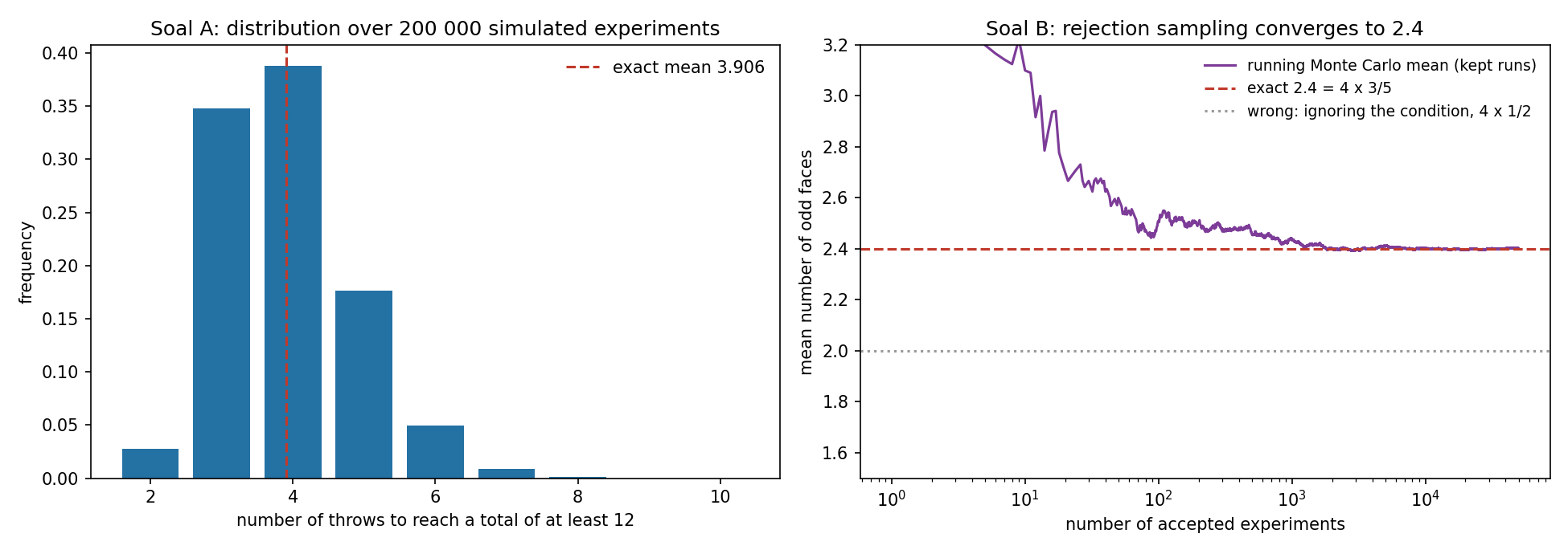
With 200 000 runs we get $3.9036 \pm 0.0042$ (95 % interval).

Exact check. Let $E_s$ be the expected number of additional throws when the current total is $s$. Then $E_s = 0$ for $s \ge 12$, and conditioning on the next throw gives

$$E_s = 1 + \frac16 \sum_{k=1}^{6} E_{s+k}, \qquad s = 11, 10, \dots, 0 .$$

Computing backwards from $s = 11$ with exact fractions gives

$$E_0 = \frac{1\,417\,221\,463}{362\,797\,056} \approx 3.9064 ,$$

inside the Monte Carlo interval.

A sanity check worth knowing. A naive guess is $12 / 3.5 \approx 3.43$ throws, since each throw adds 3.5 on average. It is too low because the last throw overshoots: when you stop, the total is between 12 and 17. Wald's identity makes this exact: $\mathbf E[\text{total at stop}] = 3.5 \times \mathbf E[\text{throws}]$, so the average final total is $3.5 \times 3.906 \approx 13.67$, i.e. an average overshoot of 1.67 above 12.

Soal B: odd faces, given that the first 6 came on throw 5

Simulation by rejection. Run the experiment "throw until a 6" many times and keep only the runs of length exactly 5:

kept = []
while len(kept) < 50_000:
    faces = []
    while True:
        f = random.randint(1, 6); faces.append(f)
        if f == 6: break
    if len(faces) == 5:                       # the condition of the question
        kept.append(sum(f % 2 for f in faces))
print(np.mean(kept))

We get $2.4018 \pm 0.0086$ from 50 000 accepted runs. Only about 8 % of the runs are accepted, since $P(\text{first 6 at throw 5}) = (5/6)^4 \cdot (1/6) \approx 0.080$. Rejection sampling is simple and always correct, but it wastes most of the work when the condition is rare.

Exact value. The condition says: throws 1 to 4 are not 6, and throw 5 is a 6. Since the throws are independent, conditioning on "not a 6" makes each of the first four throws uniform on $\{1, 2, 3, 4, 5\}$. Three of those five faces are odd, so each of the first four throws is odd with probability $3/5$. The fifth throw is a 6, which is even. By linearity of expectation,

$$\mathbf E[\text{odd faces} \mid X = 5] = 4 \times \frac35 = \frac{12}{5} = 2.4 .$$

The same reasoning gives a much faster simulation, with no rejection at all: draw four faces uniformly from 1 to 5 and count the odd ones. It returns 2.4021.

The classic trap is to ignore the conditioning: "4 throws before the 6, each odd with probability 1/2", which gives 2. Knowing that a throw was not a 6 removes one even face, so odd faces become more likely ($3/5 > 1/2$). Conditioning changes the distribution of the other throws, and a simulation that does not enforce the condition answers a different question.

Results

question	Monte Carlo (95 % interval)	exact
worked example (throws until even)	about 2	$1/p = 2$
Soal A	$3.9036 \pm 0.0042$ (200 000 runs)	$3.9064$
Soal B, rejection sampling	$2.4018 \pm 0.0086$ (50 000 accepted runs)	$2.4$
Soal B, direct sampling of the conditional law	$2.4021$ (200 000 runs)	$2.4$
Soal B, naive (no conditioning)		$2.0$ (wrong)

What to remember

• Always report a Monte Carlo estimate with its standard error $\sigma/\sqrt N$; it tells you how many runs you need and whether the simulation agrees with theory.
• Simulate the stopping rule exactly: the throw that crosses the threshold counts, and the overshoot is why the answer exceeds $12/3.5$.
• For a conditional expectation, either reject the runs that violate the condition or sample from the conditional law directly; never ignore the condition.
• Check simulations against small exact computations (a backwards recursion over states, linearity of expectation). They catch both coding bugs and formula slips like $1/(1-p)$ instead of $1/p$.