IOAI Training: Learn AI by solving problems

The problem in brief

In an imaginary kingdom, people keep records of their snowmen. For 1 000 weeks you get nine weekly statistics (temperature, wind speed and direction, precipitation, number of frosty days, price of carrots, a scarf-sale flag, number of action movies released, firewood consumption) and the number of snowmen counted. You must predict the count for 1 000 other weeks. The starter notebook "trains" a DummyRegressor, which always predicts the mean, and the only stated goal is to do better than it.

The data and starter notebook are in the official HAIO repository; the test labels are not public, and the Kaggle page is gone. We therefore evaluate on the starter notebook's own split of the labelled data (20 % held out, random_state=43), and all the detective work below uses only the other 80 %.

How you are scored

The metric is the root mean squared error:

\text{RMSE} = \sqrt{\frac{1}{n}\sum_{i=1}^{n} (\hat{y}_i - y_i)^2} .

It is in the unit of the target (snowmen), and squaring makes large errors dominate. The target to beat is the DummyRegressor: on the held-out split it scores 66 229, basically the standard deviation of the counts.

First look at the data

Three facts jump out in the first five minutes.

Almost half the weeks (48 %) have exactly 0 snowmen, and the others range up to 212 000. The counts are all integers.
Linear correlations are tiny. The strongest is temperature, at only $-0.15$ ; every other column is below $0.1$ in absolute value. A careless contestant would conclude "nothing predicts anything".
Plotting tells the opposite story (left panel below). Snowmen exist only between about $-21$ °C and $+7$ °C, and their number traces a clean upside-down parabola peaking near $-7.5$ °C: too warm, the snow melts; too cold, the snow is powder and nobody goes out. A correlation coefficient measures linear association, so it is blind to a hump: the rising and falling halves cancel out.

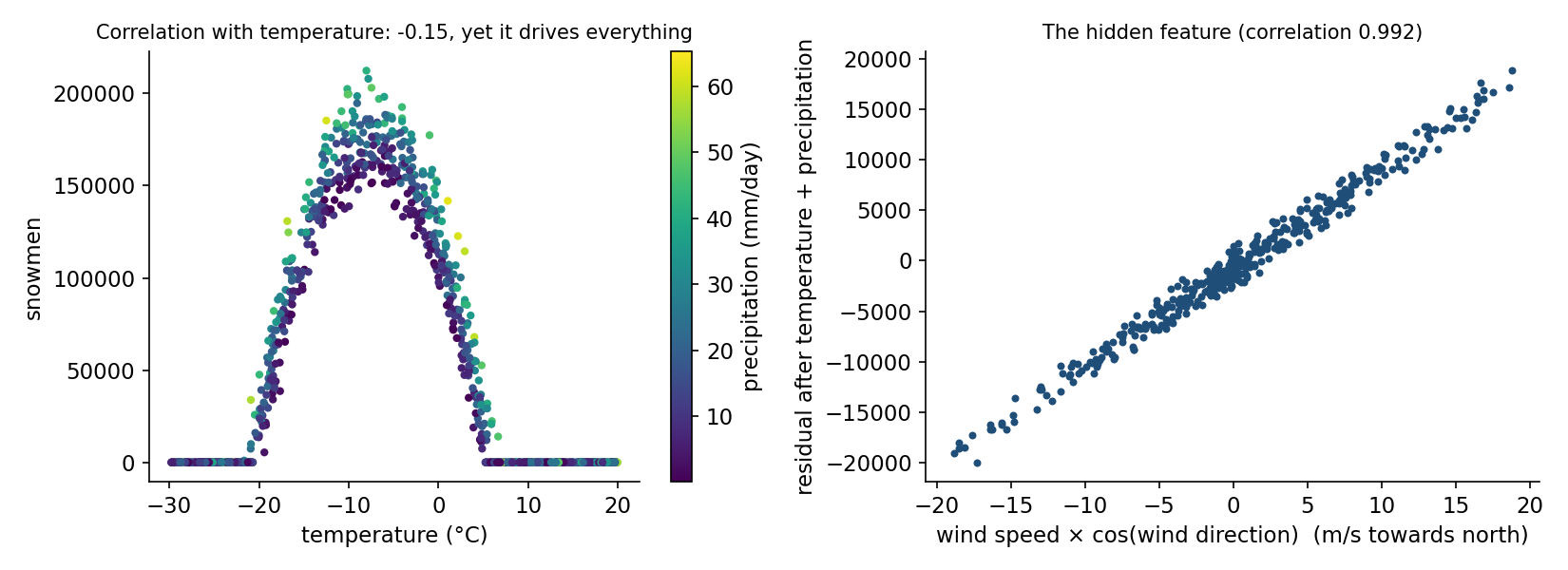
Snowmen against temperature, and the residual against the north wind

The colours add a second clue: at a given temperature, wetter weeks (yellow-green) have more snowmen. More snow, more snowmen.

A first baseline

model on the 9 raw columns	held-out RMSE
`DummyRegressor` (predict the mean)	66 229
linear regression	66 137
random forest (500 trees)	6 196
gradient boosting (800 rounds)	3 739

Linear regression is no better than the mean: it can only draw a straight line through a hump. Tree ensembles, which cut the temperature axis into pieces, already divide the error by 18. Most contestants would stop here, happy to beat the baseline by a factor of 18. But the data look synthetic: a fictional kingdom, integer counts, a perfectly smooth parabola. That suggests a hidden formula, and if we can find it we can do far better than any tree.

The key idea

Fit the formula, not a black box: model the weeks with snowmen with a linear model, read the residuals, add the feature that explains them, and repeat.

Two technical points make this work.

Fit only the weeks with snowmen. The zeros are a floor: the count cannot go negative, so the true process looks like $y = \max(0, g(x))$ . Inside the zero region, $g(x)$ is some negative number that we never see. Fitting a linear model to the zeros would bend it. So we fit $g$ on the 417 positive training weeks, and predict $\max(0, \hat{g}(x))$ everywhere.
Let the residuals point to the next feature. After each fit, compute the residuals $r = y - \hat{g}(x)$ and find which candidate feature correlates most with them.

Here is the whole investigation, every step decided on the training part only:

step	features of $g$	train residual std	strongest correlate of the residual	held-out RMSE
1	$T$ , $T^2$	14 885	precipitation, $+0.866$	10 181
2	+ precipitation $P$	7 323	$W\cos\theta$ , $+0.992$	5 808
3	+ north wind $W\cos\theta$	481	frost days $\ge 4$ , $+0.985$	356
4	+ $[\text{frost days} \ge 4]$	27.2	action movies, $-0.997$	19.0
5	+ action movies $M$	0.29	scarf flag, $-0.04$ (nothing left)	0.22

Each step needed a small idea:

Step 2 → 3: the wind. Wind speed and direction show no correlation with the residual separately. But a direction measured "relative to north" in radians invites a vector reading: the north-south component of the wind is $W\cos\theta$ . Its correlation with the residual is 0.992 (right panel above): a perfectly straight line. Speed and direction were only useful together, which no correlation table of single columns could reveal.
Step 3 → 4: a threshold. The residual grouped by number of frosty days is about $-590$ for 1 to 3 days and about $+390$ for 4 to 7 days, flat within each group. That is a step, not a slope, so the right feature is the indicator $[\text{frost days} \ge 4]$ .
Step 4 → 5: the residual is then almost perfectly (anti)correlated with the number of action movies: each one costs about 16 snowmen (people stay at the cinema?).

After step 5 the residual standard deviation is 0.29. That is exactly the standard deviation of a rounding error: a value spread uniformly over $[-0.5, 0.5]$ has standard deviation $1/\sqrt{12} \approx 0.289$ . In other words, nothing is left but the rounding to whole snowmen. Carrot prices, scarf sales and firewood play no role at all (they are decoys).

The recovered formula, with coefficients that land on round numbers:

g = 100\,171 - 15\,000\,T - 1\,000\,T^2 + 1\,000\,P + 1\,000\,W\cos\theta + 1\,000\,[F \ge 4] - 16\,M ,

\text{snowmen} = \operatorname{round}\big(\max(0, g)\big).

Completing the square, $-15\,000\,T - 1\,000\,T^2 = 56\,250 - 1\,000\,(T + 7.5)^2$ : the hump is centred at exactly $-7.5$ °C, as the plot suggested.

The full solution

Add three engineered features: $T^2$ , the north wind $W\cos\theta$ and the indicator $[\text{freeze days} \ge 4]$ .
Fit an ordinary linear regression on the training weeks with at least one snowman, using $T, T^2, P, W\cos\theta, [F \ge 4], M$ .
Predict $\max(0, \hat{g})$ and round to the nearest integer.

f["T2"] = d.temperature ** 2
f["north_wind"] = d.wind_speed * np.cos(d.wind_direction)
f["freeze_4plus"] = (d.freeze_days >= 4).astype(int)
lin = LinearRegression().fit(F.iloc[pos][cols], y[pos])          # pos = weeks with snowmen
pred = np.round(np.clip(lin.predict(F_test[cols]), 0, None))

Fitted coefficients: $-14\,999.99$ , $-1\,000.00$ , $+1\,000.00$ , $+1\,000.00$ , $+999.99$ , $-15.98$ , intercept $100\,171.0$ .

Results

approach	held-out RMSE
starter `DummyRegressor`	66 229
linear regression, raw columns	66 137
random forest, raw columns	6 196
gradient boosting, raw columns	3 739
clip(linear: $T, T^2$ )	10 181
clip(linear: + $P$ )	5 808
clip(linear: + north wind)	356
clip(linear: + frost days $\ge 4$ )	19.0
clip(linear: + action movies)	0.22
final: same, rounded to integers	0.16

Held-out RMSE of every approach

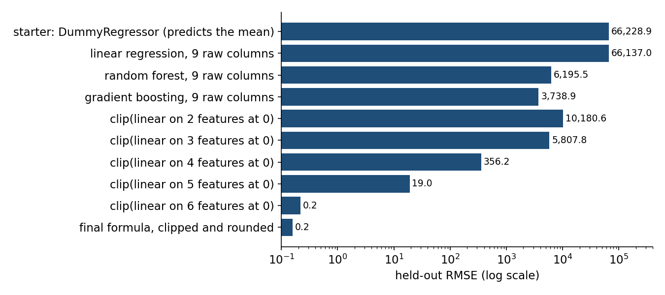
The final model reaches a held-out RMSE of 0.16 snowmen, against 66 229 for the baseline to beat: it reproduces the generating formula, and its remaining errors are a few rounding ties. Gradient boosting, the best black box, stays 20 000 times worse, because trees approximate a smooth surface with steps and need far more than 800 examples to draw a parabola, a vector component and a threshold precisely.

What to remember

Plot before you trust a correlation. Temperature has a correlation of $-0.15$ and explains most of the target: correlation only measures straight-line relations.
Residuals are a to-do list. Fit, look at what is left, find what correlates with it, add it, repeat. When the residual becomes pure noise (here the $1/\sqrt{12}$ of rounding), stop.
Think about what a column means. A direction and a speed together form a vector; a count of frosty days may act through a threshold. Physical reasoning creates the features that no single column shows.
Handle floors explicitly. When a target is clipped at 0, fit the underlying quantity on the unclipped part and clip the prediction.
Suspect synthetic data. Round coefficients, integer targets, decoy columns: on generated data, recovering the formula beats any model.

"""
HAIO 2026 summer online selection, task A "Counting Snowmen": regress the weekly number of snowmen, metric RMSE.
Data: official HAIO repo, github.com/Hungarian-AI-Olympiad/HAIO-Hungarian-AI-Olympiad, 2026/nyari-online/A/adatok
(train_labeled.csv with the target, test.csv without). The target must beat the starter DummyRegressor.

We keep the starter's own split (test_size=0.2, random_state=43) as the held-out evaluation, and use only the
80 % part for every discovery. The data turn out to follow an exact hidden formula, which we recover step by step.
Run: python solution.py   (a few seconds; figures go to ./figures)
"""
import os, warnings
import numpy as np, pandas as pd
import matplotlib; matplotlib.use("Agg")
import matplotlib.pyplot as plt
from sklearn.model_selection import train_test_split
from sklearn.metrics import root_mean_squared_error as rmse
from sklearn.dummy import DummyRegressor
from sklearn.linear_model import LinearRegression
from sklearn.ensemble import RandomForestRegressor, HistGradientBoostingRegressor
warnings.filterwarnings("ignore")
D = os.environ.get("DATA_DIR", "work"); FIG = "figures"; os.makedirs(FIG, exist_ok=True)
plt.rcParams.update({"font.size": 11, "axes.spines.top": False, "axes.spines.right": False})

df = pd.read_csv(f"{D}/train_labeled.csv"); test = pd.read_csv(f"{D}/test.csv")
RAW = list(df.columns[1:-1]); y = df["Hoember"].values
tr, ev = train_test_split(np.arange(len(df)), test_size=0.2, random_state=43)   # the starter's split
print(f"share of weeks with 0 snowmen: {(y == 0).mean():.3f}; all targets are integers: {(y == np.round(y)).all()}")

def features(d):
    f = d[RAW].copy()
    f["T2"] = d.temperature ** 2                                    # snowmen need cold, but not too cold
    f["north_wind"] = d.wind_speed * np.cos(d.wind_direction)       # wind component towards north
    f["freeze_4plus"] = (d.freeze_days >= 4).astype(int)            # a threshold effect, not a slope
    return f
F, Ft = features(df), features(test)

res = []
def report(name, pred):
    res.append((name, rmse(y[ev], pred))); print(f"{name:58s} held-out RMSE {res[-1][1]:10.2f}")

report("starter: DummyRegressor (predicts the mean)", DummyRegressor().fit(F.iloc[tr][RAW], y[tr]).predict(F.iloc[ev][RAW]))
report("linear regression, 9 raw columns", LinearRegression().fit(F.iloc[tr][RAW], y[tr]).predict(F.iloc[ev][RAW]))
rf = RandomForestRegressor(500, min_samples_leaf=2, n_jobs=2, random_state=0).fit(F.iloc[tr][RAW], y[tr])
report("random forest, 9 raw columns", rf.predict(F.iloc[ev][RAW]))
hgb = HistGradientBoostingRegressor(max_iter=800, learning_rate=0.05, random_state=0).fit(F.iloc[tr][RAW], y[tr])
report("gradient boosting, 9 raw columns", hgb.predict(F.iloc[ev][RAW]))

# ---------------------------------------------------------------- detective work: fit only the weeks WITH snowmen
# (the zeros are a floor: the true formula is cut at 0, so including them would bend a linear fit)
pos = tr[y[tr] > 0]
steps = [["temperature", "T2"], ["temperature", "T2", "precipation"],
         ["temperature", "T2", "precipation", "north_wind"],
         ["temperature", "T2", "precipation", "north_wind", "freeze_4plus"],
         ["temperature", "T2", "precipation", "north_wind", "freeze_4plus", "action_movies"]]
for cols in steps:
    lin = LinearRegression().fit(F.iloc[pos][cols], y[pos])
    r = y[pos] - lin.predict(F.iloc[pos][cols])
    others = [c for c in list(F.columns) if c not in cols and c != "wind_direction"]
    best = max(others, key=lambda c: abs(np.corrcoef(F.iloc[pos][c], r)[0, 1]))
    pred = np.clip(lin.predict(F.iloc[ev][cols]), 0, None)          # snowmen cannot be negative
    report(f"clip(linear on {len(cols)} features at 0)", pred)
    print(f"     residual std on train {r.std():9.2f} | most correlated remaining feature: {best} "
          f"({np.corrcoef(F.iloc[pos][best], r)[0, 1]:+.3f})")
print("final coefficients:", dict(zip(cols, lin.coef_.round(3))), "intercept", round(lin.intercept_, 2))
final = lambda d: np.round(np.clip(lin.predict(d[cols]), 0, None))      # targets are integers
report("final formula, clipped and rounded", final(F.iloc[ev]))
pd.DataFrame({"ID": test.ID, "Hoember": final(Ft)}).to_csv("prediction.csv", index=False)

# ---------------------------------------------------------------- figures
fig, ax = plt.subplots(1, 2, figsize=(11, 4))
sc = ax[0].scatter(df.temperature, y, c=df.precipation, s=9, cmap="viridis")
plt.colorbar(sc, ax=ax[0], label="precipitation (mm/day)")
ax[0].set_xlabel("temperature (°C)"); ax[0].set_ylabel("snowmen"); ax[0].set_title(
    f"Correlation with temperature: {np.corrcoef(df.temperature, y)[0, 1]:+.2f}, yet it drives everything", fontsize=10)
lin3 = LinearRegression().fit(F.iloc[pos][steps[1]], y[pos]); r3 = y[pos] - lin3.predict(F.iloc[pos][steps[1]])
ax[1].scatter(F.iloc[pos]["north_wind"], r3, s=8, color="#1f4e79")
ax[1].set_xlabel("wind speed × cos(wind direction)  (m/s towards north)")
ax[1].set_ylabel("residual after temperature + precipitation")
ax[1].set_title(f"The hidden feature (correlation {np.corrcoef(F.iloc[pos]['north_wind'], r3)[0, 1]:.3f})", fontsize=10)
plt.tight_layout(); plt.savefig(f"{FIG}/detective.png", dpi=150); plt.close()

r = pd.DataFrame(res, columns=["model", "rmse"])
fig, ax = plt.subplots(figsize=(9, 4))
ax.barh(r.model[::-1], r.rmse[::-1], color="#1f4e79"); ax.set_xscale("log")
for i, v in enumerate(r.rmse[::-1]): ax.text(v * 1.1, i, f"{v:,.1f}", va="center", fontsize=9)
ax.set_xlabel("held-out RMSE (log scale)"); ax.set_xlim(0.1, 4e5)
plt.tight_layout(); plt.savefig(f"{FIG}/results.png", dpi=150)