IOAI Training: Learn AI by solving problems

The problem in brief

About 12 000 weather stations report every hour: temperature, "feels-like" and dew-point temperatures, wind speed and gusts, pressure, humidity, visibility, cloud cover, UV index, day/night, and a rain category from 0 (none) to 3 (heavy). The data, from the first half of January 2022, is cut into windows of 23 consecutive hours, each with an identifier. For each window you must predict the rain category of the 24th hour, the one just after the window. There are 104 836 training windows with their answer and 40 000 test windows.

The test labels are private on Kaggle and we never submitted anything. All our scores come from a stratified 80/20 split of the training windows (83 868 to train, 20 968 held out).

How you are scored

The metric is the quadratic weighted kappa (QWK) between true and predicted categories. With $O_{ij}$ the number of windows of true class $i$ predicted as $j$ , $E_{ij}$ the count expected if predictions were independent of the truth (same marginals), and weights growing with the squared distance between classes,

w_{ij} = \frac{(i-j)^2}{(K-1)^2}, \qquad \kappa = 1 - \frac{\sum_{ij} w_{ij}\,O_{ij}}{\sum_{ij} w_{ij}\,E_{ij}} .

So $\kappa = 1$ is perfect agreement, $\kappa = 0$ is chance level, and confusing "none" with "heavy" costs 9 times more than confusing two neighbouring categories. The classes are ordered, and the metric knows it.

What to aim for. On the public leaderboard, the organisers' random-forest baseline scores 0.765, the organisers' own solutions 0.901 (CatBoost) and 0.908 (neural network), and the best contestant 0.903.

First look at the data

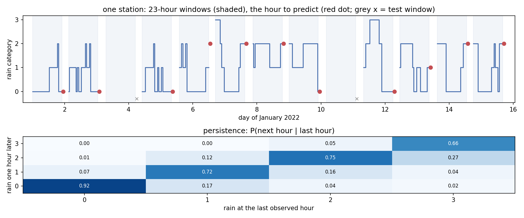
Windows of one station and the persistence of rain

Rain is very persistent. The lower panel shows, over all training windows, the category one hour after the last observed hour as a function of the last observed one: 92 % of dry hours are followed by a dry hour, and 66 to 75 % of rainy hours keep the same category. Simply repeating the last observed value ("persistence") already gives QWK 0.852, much more than the organisers' baseline.
The classes are unbalanced: 60 % "none", 23 % light, 15 % moderate, 2.5 % heavy.
The windows are pieces of one long series per station. Every station has about 12 windows (train and test mixed), and consecutive windows start 27 to 30 hours apart. A window covers hours $t_0, \dots, t_0+22$ , we predict hour $t_0+23$ , and the station's next window starts at $t_0+27$ to $t_0+30$ , so only 4 to 7 hours after the hour we must predict (upper panel, shaded areas; test windows have no line because their sensor rows are in the test file, with a grey cross where the target is hidden).
All 12 000 stations report at the same hours. At any given hour, many other stations have a window covering it.

A first baseline

The organisers' baseline keeps only the last row of each window (the 23rd hour) and trains a random forest classifier on its 14 measurements. It scores 0.765 on the leaderboard. Two things are lost: the whole recent history (is the rain starting, ending, getting heavier?) and the ordinal nature of the target (a classifier does not know that 2 lies between 1 and 3).

The key idea

Use the time structure: summarise the 23-hour history with "last value, recent change, recent level" features, treat the target as a number (an ordered category), and add the context that the data layout gives away, namely what the same station reports a few hours later and what all stations report at the target hour.

History features. For each of the 14 variables: the last three values, the differences over 1, 3 and 6 hours, the mean over the last 6 hours, and the mean, minimum and maximum over the 23 hours; plus the number of rainy hours, the maximum rain over the last 6 hours, and the hour of day of the target. Physically, rain arrives with rising humidity and cloud cover, falling visibility and pressure, so the trends carry information that the last value alone does not.
Ordinal target. A gradient-boosting regression on the category, rounded to the nearest integer, respects the ordering: a window that is half-way between "light" and "moderate" gets 1.5, not an arbitrary class. We also train a 4-class model and use its expected value $\sum_k k\,p_k$ , which is again a number on the same scale, and we average the two.
Context from the layout. The next window of the same station (identified by station and start time, train or test) starts 4 to 7 hours after the target; its first rain values, humidity and cloud cover tell us whether the rain was still there a few hours later. And the mean rain category over all stations at the target hour (and the hour before) captures the large-scale weather of that moment. These are not available to a real forecaster, but they are part of the data the organisers handed out, legitimate inside the competition, and they add about +0.008 of QWK.

Why does rounding a regression suit QWK? The penalty grows like $(i-j)^2$ , which is exactly the squared error on the class index. A regression trained on squared error minimises the same kind of loss, so its rounded output is naturally close to what QWK rewards. We also tried the classic trick of tuning the three rounding thresholds on held-out data (fitted on one half of the validation set, scored on the other); here it brought nothing (0.9066 against 0.9073 with plain rounding), because the regression is already well calibrated.

The full solution

Sort the rows by window and hour and reshape them into an array of shape (windows, 23 hours, 14 variables); compute the 143 history features with NumPy.
Order each station's windows by start time and attach the first 4 hours of the next window (rain, humidity, cloud), its first pressure value, the gap in hours, and the last rain value of the previous window.
Attach the mean rain, humidity and number of reporting stations at the target hour, and the mean rain one hour earlier.
Train LightGBM twice (63 leaves, learning rate 0.05, row and column subsampling): a regression (about 1 500 trees) and a 4-class classifier (about 350 trees); the numbers of trees come from early stopping on the held-out split.
Prediction $= \text{round}\big(\tfrac12(\hat y_{\text{reg}} + \sum_k k\,\hat p_k)\big)$ , clipped to 0..3.

ev = cls.predict(Xb) @ np.arange(4)          # expected category under the class probabilities
pred = np.clip(np.round((reg.predict(Xb) + ev) / 2), 0, 3).astype(int)

Building the features takes a few seconds, the two models about two minutes on 2 CPU threads.

Results

approach (held-out 20 % of training windows unless stated)	QWK
organisers' random forest on the last row (public leaderboard)	0.765
persistence: repeat the last observed category	0.852
LightGBM regression, 23-hour history features, rounded	0.899
+ next window of the same station	0.904
+ all-station means at the target hour	0.907
same, rounding thresholds tuned on half of the validation set	0.907
4-class LightGBM, most probable class	0.907
4-class LightGBM, expected value rounded	0.908
average of regression and expected value, rounded (final)	0.909

The final model reaches QWK 0.909 on 20 968 held-out windows, at the level of the organisers' best solution on the public leaderboard (0.908) and above the best contestant (0.903). The leaderboard uses the hidden test windows, so this comparison is indicative, but with 21 000 windows our estimate is precise to about $\pm 0.003$ .

The remaining errors are almost all between neighbouring categories: in the held-out confusion matrix, only about 50 of 20 968 windows (0.2 %) are off by two classes or more. The hardest case is the onset of rain after a dry window, which no feature of the past can announce with certainty.

What to remember

Always try persistence first on a time series. Here "tomorrow looks like today" (or rather "the next hour looks like this one") gave 0.852 with no model at all, far above the official baseline.
Summarise a window with last values, short-range differences and recent means. Trends are often more informative than levels.
Respect the order of the classes. For an ordinal target scored by QWK, a rounded regression (or the expected value of a classifier) is a natural fit, because the squared penalty of QWK matches the squared error.
Look at how the data was cut. Windows of one long series, with gaps of a few hours, mean that neighbouring windows carry information about each other's targets; exploring identifiers and timestamps is part of the job.

"""Tenerife camp day 2, weather prediction: predict the rain category (0-3) of the 24th hour from
23 hourly sensor rows of a weather station. Metric: quadratic weighted kappa (QWK).

Files train_weather.parquet, test_weather.parquet, train_target_weather.parquet and
sample_submission_weather.csv from the Kaggle competition, in the working folder. Test labels are
private: `python solution.py holdout` scores a stratified 80/20 split of the 104 836 training chunks,
`python solution.py final` trains on all of them and writes submission.csv.

Pipeline
  1. each chunk -> a 23 x 14 array (hours x variables) -> summary features (last values, short-range
     differences, means/extremes over the window, 6-hour means);
  2. context features: the first hours of the NEXT 23-hour window of the same station (it starts
     4 to 7 hours after the target hour) and the mean rain of all stations at the target hour;
  3. LightGBM regression on the category + LightGBM multiclass (expected value), averaged and rounded.
"""
import sys, warnings
warnings.filterwarnings("ignore")
import numpy as np, pandas as pd
VARS = ["tempc", "feelslikec", "windspeed_kph", "windgust_kph", "pressure_mb", "humidity", "visibility_km", "cloud",
        "heatindexc", "dewpointc", "windchillc", "uvindex", "isday", "rain"]

def build(use_next=True, use_cross=True):
    tr = pd.read_parquet("train_weather.parquet"); te = pd.read_parquet("test_weather.parquet")
    y = pd.read_parquet("train_target_weather.parquet").set_index("chunk_id").rain
    d = pd.concat([tr, te], ignore_index=True); del tr, te
    d["ts"] = (pd.to_datetime(d.date) - pd.Timestamp("2022-01-01")).dt.days * 24 + d.time
    d = d.sort_values(["chunk_id", "ts"]).reset_index(drop=True)
    ids = d.chunk_id.values[::23]; N = len(ids)
    A = d[VARS].to_numpy(np.float32).reshape(N, 23, len(VARS))       # chunk x hour x variable
    st = d.stationid.values[::23]; t0 = d.ts.values[::23]
    F = {}
    for j, v in enumerate(VARS):
        x = A[:, :, j]
        F[f"{v}_last"] = x[:, -1]; F[f"{v}_l2"] = x[:, -2]; F[f"{v}_l3"] = x[:, -3]
        F[f"{v}_mean"] = x.mean(1); F[f"{v}_max"] = x.max(1); F[f"{v}_min"] = x.min(1)
        F[f"{v}_d1"] = x[:, -1] - x[:, -2]; F[f"{v}_d3"] = x[:, -1] - x[:, -4]; F[f"{v}_d6"] = x[:, -1] - x[:, -7]
        F[f"{v}_mean6"] = x[:, -6:].mean(1)
    F["rain_n_pos"] = (A[:, :, -1] > 0).sum(1); F["rain_last6_max"] = A[:, -6:, -1].max(1)
    F["target_hour"] = (t0 + 23) % 24; F["station"] = st
    X = pd.DataFrame(F); X["chunk_id"] = ids; X["t0"] = t0
    if use_next:   # neighbouring chunks of the same station (the data are cut into 23 h windows with gaps)
        o = X.sort_values(["station", "t0"]).index.values
        S = X.loc[o, ["station", "t0"]].reset_index(drop=True)
        R = A[o, :, -1]; H = A[o, :, VARS.index("humidity")]; C = A[o, :, VARS.index("cloud")]; P = A[o, :, VARS.index("pressure_mb")]
        same_next = (S.station.values[1:] == S.station.values[:-1])
        def nxt(arr, k):
            out = np.full(len(o), np.nan, np.float32); out[:-1] = np.where(same_next, arr[1:, k], np.nan); return out
        def prv(arr, k):
            out = np.full(len(o), np.nan, np.float32); out[1:] = np.where(same_next, arr[:-1, k], np.nan); return out
        G = {}
        gap = np.full(len(o), np.nan, np.float32); gap[:-1] = np.where(same_next, S.t0.values[1:] - S.t0.values[:-1] - 23, np.nan)
        G["next_gap_h"] = gap
        for k in range(4):
            G[f"next_rain_{k}"] = nxt(R, k); G[f"next_hum_{k}"] = nxt(H, k); G[f"next_cloud_{k}"] = nxt(C, k)
        G["next_pres_0"] = nxt(P, 0)
        G["prev_rain_last"] = prv(R, -1)
        for k, v in G.items():
            col = np.empty(len(o), np.float32); col[o] = v; X[k] = col
    if use_cross:  # what the other stations report at the target hour itself
        r = d[["ts", "rain", "humidity", "cloud"]].groupby("ts").agg(["mean", "size"])
        tt = t0 + 23
        X["cross_rain_mean"] = pd.Series(tt).map(r[("rain", "mean")]).values
        X["cross_n"] = pd.Series(tt).map(r[("rain", "size")]).values
        X["cross_hum_mean"] = pd.Series(tt).map(r[("humidity", "mean")]).values
        X["cross_rain_prevh"] = pd.Series(tt - 1).map(r[("rain", "mean")]).values
    X["y"] = X.chunk_id.map(y)
    return X


import lightgbm as lgb
from sklearn.metrics import cohen_kappa_score
from sklearn.model_selection import train_test_split

DROP = ["chunk_id", "t0", "y", "station"]
BASE = dict(learning_rate=0.05, num_leaves=63, min_child_samples=50, subsample=0.8, subsample_freq=1,
            colsample_bytree=0.7, n_jobs=2, verbose=-1)


def fit_predict(Xa, ya, Xb, n_reg=1500, n_cls=350):
    reg = lgb.train(dict(BASE, objective="regression"), lgb.Dataset(Xa, ya), n_reg)
    cls = lgb.train(dict(BASE, objective="multiclass", num_class=4), lgb.Dataset(Xa, ya), n_cls)
    ev = cls.predict(Xb) @ np.arange(4)                  # expected category under the class probabilities
    return np.clip(np.round((reg.predict(Xb) + ev) / 2), 0, 3).astype(int)


if __name__ == "__main__":
    mode = sys.argv[1] if len(sys.argv) > 1 else "holdout"
    X = build()
    cols = [c for c in X.columns if c not in DROP]
    L, T = X[X.y.notna()].reset_index(drop=True), X[X.y.isna()].reset_index(drop=True)
    y = L.y.values.astype(int)
    if mode == "holdout":
        tr, va = train_test_split(np.arange(len(L)), test_size=0.2, random_state=0, stratify=y)
        pred = fit_predict(L.loc[tr, cols], y[tr], L.loc[va, cols])
        print("persistence QWK", round(cohen_kappa_score(y[va], L.rain_last.values[va].astype(int), weights="quadratic"), 4))
        print("holdout QWK", round(cohen_kappa_score(y[va], pred, weights="quadratic"), 4))
    else:
        pred = fit_predict(L[cols], y, T[cols], n_reg=1650, n_cls=390)   # ~10 % more trees for 25 % more data
        sub = pd.read_csv("sample_submission_weather.csv")
        sub[sub.columns[1]] = sub.chunk_id.map(dict(zip(T.chunk_id, pred)))
        sub.to_csv("submission.csv", index=False)
        print("wrote submission.csv", sub[sub.columns[1]].value_counts().to_dict())

Tenerife day2 - weather prediction