IOAI Training: Learn AI by solving problems

The problem in brief

Dermatologists photograph suspicious skin spots through a dermoscope, a magnifier with its own lighting. You receive 4 000 such photographs (224 × 224 pixels) from the public HAM10000 collection, each labelled with one of 7 diagnoses: melanoma (mel), basal cell carcinoma (bcc), actinic keratosis (akiec), benign keratosis (bkl), the ordinary mole or naevus (nv), dermatofibroma (df) and vascular lesion (vasc). Each image also comes with three facts about the patient: age, sex and where on the body the lesion is. You must diagnose 1 000 test images, using both the picture and the patient data.

The test labels are private on Kaggle and we never submitted anything. The scores below come from our own validation on the 4 000 labelled images: 5-fold cross-validation for the cheap models, and one stratified 80/20 split (3 200 for training, 800 held out) for the fine-tuned network, which takes 15 minutes per run.

How you are scored

The metric is the weighted F1 score. For each class $c$ compute $\text{F1}_c = 2P_cR_c/(P_c+R_c)$ from its precision and recall, then average with weights equal to the class frequencies $n_c/n$ :

\text{F1}_{\text{weighted}} = \sum_{c} \frac{n_c}{n}\,\text{F1}_c .

The weighting matters a lot here. Moles are 66 % of the data, so their F1 counts for two thirds of the score, while the 43 dermatofibromas count for 1 %. A model that is excellent on moles and mediocre on rare diseases can still score well. (Medically you would choose a different metric, one that punishes missed melanomas; the competition did not.)

What to aim for. The public leaderboard has a best weighted F1 of 0.876. There is no official threshold.

First look at the data

Two images per class

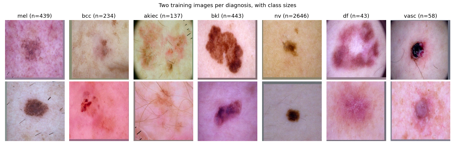
Strong class imbalance: 2 646 moles, then 443 benign keratoses and 439 melanomas, down to 58 vascular lesions and 43 dermatofibromas. Always predicting "mole" already gives a weighted F1 of 0.527.
The images vary in colour and zoom, many have hairs, rulers or the dark circle of the dermoscope, and several have grey padding along one or two edges. A lesion has no natural orientation: a mole rotated by 90° is still a mole.
Patient data carries real signal. Moles are the only common class seen in teenagers and young adults, while actinic keratoses and carcinomas appear almost only after 40 (left panel below). A logistic regression on age, sex and site alone reaches 0.562, better than the majority guess.

A first baseline

The quickest strong baseline in vision: use a pretrained network as a fixed feature extractor. We pass every image (and its three mirror images, averaged) through two ImageNet-pretrained models, ConvNeXt-Tiny and the self-supervised DINOv2-Small, keep their final 768- and 384-dimensional feature vectors, and train a logistic regression on top. No network weight is changed, so it takes three minutes in total.

frozen features + logistic regression (5-fold CV)	image only	image + age, sex, site
DINOv2-Small	0.759	0.792
ConvNeXt-Tiny	0.763	0.793
both concatenated		0.801

Two lessons already. Pretrained features are a huge step (0.53 to 0.76). And adding the three patient columns, standardised and concatenated with the image features (scaled up so the regulariser does not drown them among 1 152 image features), is worth +0.03: the "multimodal" part of the title is not decoration.

The key idea

Fuse the patient data with the image inside one network, and fine-tune the upper part of a pretrained CNN while respecting what a dermoscopic image is: a picture with no orientation, varying zoom and varying light.

Frozen ImageNet features describe dogs and cars well, skin less so. Fine-tuning lets the higher layers specialise in pigment networks, vessels and borders. Three design choices make it work with only 3 200 training images:

Freeze the bottom, train the top. The stem and the first two stages of ConvNeXt compute generic edges and textures that transfer well; only the last two stages (about 90 % of the parameters but the most task-specific) are trained. This also halves the memory and time.
Different learning rates for old and new parts. The pretrained stages get $10^{-4}$ , the freshly initialised head and tabular branch $2 \times 10^{-3}$ . Our first attempt used one learning rate everywhere and stalled at a training loss near the entropy of the class frequencies: the random head was learning too slowly and the backbone was being pushed around by meaningless gradients.
Augment with the symmetries of the problem. Random horizontal and vertical flips plus rotations by multiples of 90° generate the 8 orientations of the square (all equally plausible for a lesion), a random zoom of 75 to 100 % mimics different magnifications, and brightness and contrast jitter of ±15 % mimics different lighting. At test time we average the predictions over 4 such views.

The patient data enters through a small branch: age, age², one-hot sex and one-hot site go through a 32-unit layer, and its output is concatenated with the 768 image features before the final linear classifier:

p(\text{diagnosis}) = \operatorname{softmax}\!\Big(W\,\big[\,f_{\text{CNN}}(\text{image}) \;;\; \operatorname{ReLU}(A\,t + b)\,\big]\Big).

The network can then learn interactions such as "this looks like a keratosis, but the patient is 18, so it is probably a mole".

The full solution

Model A (frozen): DINOv2-S and ConvNeXt-T features, flip-averaged, concatenated with the patient features, logistic regression with $C = 0.02$ .
Model B (fine-tuned): ConvNeXt-T (ImageNet-22k pretrained, safetensors weights) with the tabular branch, stem and stages 1-2 frozen, AdamW (weight decay 0.05), one-cycle schedule over 8 epochs, batch 16, label smoothing 0.1, dropout 0.3 in the head, augmentation as above, 4-view test-time averaging. Gradient checkpointing keeps the GPU memory under 2 GB.
Blend: $0.7\,p_B + 0.3\,p_A$ , predict the most probable class.

x = (augment(to_tensor(Xi[b])) - MEAN) / STD          # flips, 90-degree turns, zoom, lighting
loss = F.cross_entropy(m(x, tabular[b]), y[b], label_smoothing=0.1)

One epoch takes 1 to 2 minutes on the Apple GPU (shared with other jobs).

Results

approach	evaluation	weighted F1
always "mole"	5-fold CV	0.527
age, sex, site only (logistic regression)	5-fold CV	0.562
frozen DINOv2-S, image only	5-fold CV	0.759
frozen ConvNeXt-T + patient data	5-fold CV	0.793
frozen DINOv2-S + ConvNeXt-T + patient data (model A)	5-fold CV / 80-20 split	0.801 / 0.779
fine-tuning the whole network, one learning rate (failed)	80-20 split	0.56 to 0.68
fine-tuned ConvNeXt-T + patient branch (model B)	80-20 split	0.805
blend 0.7 B + 0.3 A (final)	80-20 split	0.806

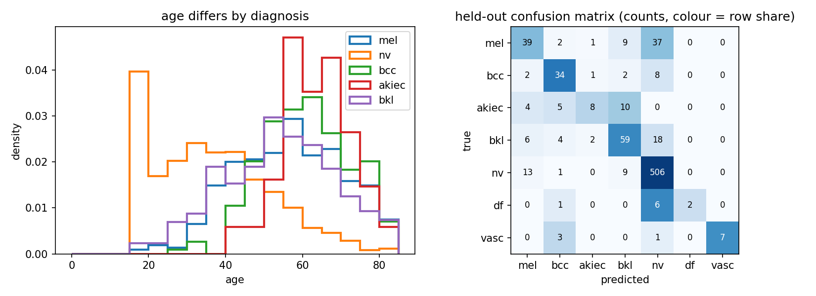
Age by diagnosis and the confusion matrix

Our final model reaches a weighted F1 of 0.806 on the 800 held-out images, well above the baselines but clearly below the best public leaderboard score of 0.876. The comparison is not exact (different images, and an 800-image split has a standard error of about 0.014), but the gap is real, so this problem is not fully solved by our pipeline. The fine-tuned network was still improving at the last epoch (held-out F1 0.71, 0.74, 0.79, 0.81 after epochs 2, 4, 6, 8); a longer schedule, unfreezing the lower stages in a second phase, higher input resolution, or an ensemble of several backbones are the natural next steps that we could not afford within the compute budget of this correction.

The confusion matrix shows where the errors are. Moles are recognised 96 % of the time. The weak spot is melanoma versus mole: 37 of 88 held-out melanomas are called moles, the most dangerous mistake of all and a famously hard distinction even for experts. Actinic keratoses are confused with benign keratoses (both are scaly, sun-damaged skin), and 6 of 9 dermatofibromas are called moles. Each of these rare classes weighs little in the weighted F1, which is why the score stays above 0.8 despite them.

What to remember

Start with frozen pretrained features and a linear model. In three minutes it reached 0.80, which tells you how much any expensive fine-tuning still has to add.
Small tabular side-information is worth fusing. Three columns (age, sex, site) added 0.03 of F1 on top of strong image features, because some diagnoses are nearly impossible at certain ages.
When fine-tuning, give the new head a larger learning rate than the pretrained body, and consider freezing the lowest layers. One learning rate for everything made our first run stall.
Choose augmentations that are true symmetries of the data. Lesions have no up or down, so the 8 rotations and mirrors of the square are free extra data, at training and at test time.
Read the metric's weights. A frequency-weighted F1 is dominated by the majority class; a model can look good while missing many melanomas, so always inspect the confusion matrix.

"""Multimodal skin-lesion classification (Cyprus AI Camp 2026), metric = weighted F1.

Data: the competition's .npy files (train/test images 224x224, tabular [age, sex, site], labels)
in the working folder; ImageNet weights as safetensors in ./w (pickle-free):
  timm/convnext_tiny.fb_in22k_ft_in1k  -> w/convnext_tiny.safetensors
  timm/vit_small_patch14_dinov2.lvd142m -> w/dinov2_s.safetensors
Test labels are private: `python solution.py holdout` scores a stratified 80/20 split,
`python solution.py final` trains on everything and writes submission.csv.

Two views of each image, fused with the patient data, then averaged:
  A. frozen features (DINOv2-S + ConvNeXt-T, flip-averaged) + age/sex/site -> logistic regression;
  B. ConvNeXt-T fine-tuned end to end (stem + first 2 stages frozen), tabular branch in the head,
     dihedral augmentation + zoom + brightness/contrast, 4-view test-time augmentation.
Final probabilities = 0.7 B + 0.3 A.
"""
import os, sys, math
os.environ.setdefault("OMP_NUM_THREADS", "2")
import numpy as np, torch, timm, torch.nn as nn, torch.nn.functional as F
import pandas as pd
from safetensors.torch import load_file
from sklearn.linear_model import LogisticRegression
from sklearn.preprocessing import StandardScaler
from sklearn.model_selection import train_test_split
from sklearn.metrics import f1_score

torch.set_num_threads(2); torch.manual_seed(0); np.random.seed(0)
DEV = "mps" if torch.backends.mps.is_available() else "cpu"
if DEV == "mps":
    torch.mps.set_per_process_memory_fraction(0.09)      # keep the GPU share under ~2 GB
CLASSES = ["mel", "bcc", "akiec", "bkl", "nv", "df", "vasc"]
MEAN = torch.tensor([0.485, 0.456, 0.406], device=DEV).view(1, 3, 1, 1)
STD = torch.tensor([0.229, 0.224, 0.225], device=DEV).view(1, 3, 1, 1)
EPOCHS, BS, LR = 8, 16, 1e-4

Xi = np.load("train_images.npy", mmap_mode="r"); Xt = np.load("test_images.npy", mmap_mode="r")
y = np.load("train_labels.npy"); T = np.load("train_tabular.npy"); Tt = np.load("test_tabular.npy")


def tab(T):   # age (and age^2), one-hot sex (2) and anatomical site (6)
    age = T[:, [0]] / 100
    return np.hstack([age, age ** 2, np.eye(2)[T[:, 1].astype(int)], np.eye(6)[T[:, 2].astype(int)]]).astype(np.float32)


def backbone(name, arch):
    kw = dict(dynamic_img_size=True) if "vit" in arch else {}
    m = timm.create_model(arch, pretrained=False, num_classes=0, **kw)
    m.load_state_dict({k: v for k, v in load_file(f"w/{name}.safetensors").items() if not k.startswith("head.fc")},
                      strict=False)
    return m


def to_tensor(arr):
    return torch.from_numpy(np.array(arr)).permute(0, 3, 1, 2).float().div(255).to(DEV)


# ---------------- A. frozen features + logistic regression ----------------
def frozen_features(X):
    feats = []
    for name, arch in [("dinov2_s", "vit_small_patch14_dinov2"), ("convnext_tiny", "convnext_tiny")]:
        m, out = backbone(name, arch).eval().to(DEV), []
        with torch.no_grad():
            for i in range(0, len(X), 32):
                x = (to_tensor(X[i:i + 32]) - MEAN) / STD
                out.append((sum(m(v) for v in [x, x.flip(3), x.flip(2), x.flip(2).flip(3)]) / 4).cpu().numpy())
        feats.append(np.concatenate(out))
        del m
        if DEV == "mps": torch.mps.empty_cache()
    return np.hstack(feats)


def model_a(Fa, Ta, ya, Fb, Tb):
    A, B = np.hstack([Fa, 3 * tab(Ta)]), np.hstack([Fb, 3 * tab(Tb)])
    s = StandardScaler().fit(A)
    return LogisticRegression(C=0.02, max_iter=3000).fit(s.transform(A), ya).predict_proba(s.transform(B))


# ---------------- B. fine-tuned ConvNeXt with a tabular branch ----------------
class Net(nn.Module):
    def __init__(self):
        super().__init__()
        self.b = backbone("convnext_tiny", "convnext_tiny")
        self.b.set_grad_checkpointing(True)                     # trades compute for memory
        for p in list(self.b.stem.parameters()) + list(self.b.stages[0].parameters()) + list(self.b.stages[1].parameters()):
            p.requires_grad_(False)                             # generic low-level filters stay frozen
        self.t = nn.Sequential(nn.Linear(10, 32), nn.ReLU())
        self.h = nn.Sequential(nn.Dropout(0.3), nn.Linear(768 + 32, 7))

    def forward(self, x, t):
        return self.h(torch.cat([self.b(x), self.t(t)], 1))


def augment(x):
    # a lesion has no "up": any rotation / mirror is a valid image; plus zoom and lighting changes
    if np.random.rand() < 0.5: x = x.flip(3)
    if np.random.rand() < 0.5: x = x.flip(2)
    x = torch.rot90(x, np.random.randint(4), (2, 3))
    n = int(224 * np.random.uniform(0.75, 1)); i, j = np.random.randint(0, 224 - n + 1, 2)
    x = F.interpolate(x[:, :, i:i + n, j:j + n], size=(224, 224), mode="bilinear", align_corners=False)
    b = torch.empty(len(x), 1, 1, 1, device=DEV).uniform_(0.85, 1.15)
    c = torch.empty(len(x), 1, 1, 1, device=DEV).uniform_(0.85, 1.15)
    mu = x.mean((1, 2, 3), keepdim=True)
    return (((x - mu) * c + mu) * b).clamp(0, 1)


def model_b(idx_train, Xb, Tb):
    m = Net().to(DEV)
    head = list(m.t.parameters()) + list(m.h.parameters())
    opt = torch.optim.AdamW([{"params": [p for p in m.b.parameters() if p.requires_grad], "lr": LR},
                             {"params": head, "lr": 20 * LR}], weight_decay=0.05)   # fresh head learns faster
    steps = EPOCHS * math.ceil(len(idx_train) / BS)
    sched = torch.optim.lr_scheduler.OneCycleLR(opt, max_lr=[LR, 20 * LR], total_steps=steps, pct_start=0.1)
    Ttr, yt = torch.tensor(tab(T)), torch.tensor(y)
    for ep in range(EPOCHS):
        m.train()
        perm = np.random.permutation(idx_train)
        for i in range(0, len(perm), BS):
            b = np.sort(perm[i:i + BS])
            x = (augment(to_tensor(Xi[b])) - MEAN) / STD
            loss = F.cross_entropy(m(x, Ttr[b].to(DEV)), yt[b].to(DEV), label_smoothing=0.1)
            opt.zero_grad(); loss.backward(); opt.step(); sched.step()
        if DEV == "mps": torch.mps.empty_cache()
        print(f"epoch {ep} done", flush=True)
    m.eval(); out = []
    if DEV == "mps": torch.mps.empty_cache()
    Tbt = torch.tensor(tab(Tb))
    with torch.no_grad():
        for i in range(0, len(Xb), 16):
            x = (to_tensor(Xb[i:i + 16]) - MEAN) / STD; t = Tbt[i:i + 16].to(DEV)
            out.append((sum(F.softmax(m(v, t), 1) for v in [x, x.flip(3), x.flip(2), torch.rot90(x, 1, (2, 3))]) / 4).cpu().numpy())
    return np.concatenate(out)


if __name__ == "__main__":
    mode = sys.argv[1] if len(sys.argv) > 1 else "holdout"
    Ftr = frozen_features(Xi)
    if mode == "holdout":
        tr, ho = train_test_split(np.arange(len(y)), test_size=0.2, stratify=y, random_state=0)
        ho = np.sort(ho)
        Pa = model_a(Ftr[tr], T[tr], y[tr], Ftr[ho], T[ho])
        Pb = model_b(tr, Xi[ho], T[ho])
        for name, P in [("A frozen+LR", Pa), ("B fine-tuned", Pb), ("0.7 B + 0.3 A", 0.7 * Pb + 0.3 * Pa)]:
            print(name, "weighted F1", round(f1_score(y[ho], P.argmax(1), average="weighted"), 4))
    else:
        Fte = frozen_features(Xt)
        Pa = model_a(Ftr, T, y, Fte, Tt)
        Pb = model_b(np.arange(len(y)), Xt, Tt)
        pred = (0.7 * Pb + 0.3 * Pa).argmax(1)
        ids = np.load("test_ids.npy", allow_pickle=True)
        pd.DataFrame({"image_id": ids, "diagnosis": [CLASSES[i] for i in pred]}).to_csv("submission.csv", index=False)
        print("wrote submission.csv")

Multimodal Skin Lesion Classification