IOAI Training: Learn AI by solving problems

The problem in brief

You are handed a BERT model that was fine-tuned to tell whether a tweet is neutral, positive or negative. A mishap damaged its token-embedding matrix (the table that turns each of the 30 522 vocabulary pieces into a 768-dimensional vector); every other weight, attention layers and classification head included, is intact. Your job is to repair that matrix so the model classifies sentiment well again, then label 2 500 test tweets. Two restrictions: no other pretrained transformer or LLM, and no outside data. All you get is the broken model and 2 500 labelled tweets (called the "validation" set by the organisers) plus the 2 500 unlabelled test tweets.

The test labels are private on Kaggle and we never submitted anything. Every score below is measured on the 2 500 labelled tweets, by 5-fold cross-validation: the repair is learned on 4/5 of the tweets and scored on the remaining fifth, five times.

How you are scored

The organisers' baseline notebook scores the predictions with the macro-averaged F1: compute the F1 of each of the three classes, then take the plain mean,

\text{F1}_c = \frac{2\,P_c R_c}{P_c + R_c}, \qquad \text{macro-F1} = \frac{1}{3}\sum_{c} \text{F1}_c ,

where $P_c$ and $R_c$ are the precision and recall of class $c$ . A model that ignores one class loses a third of the score, whatever the class sizes.

What to aim for. The public leaderboard (21 entries) has a best score of 0.616 and a median of 0.538. There is no official pass threshold.

First look at the data

Before repairing anything, find out what "damaged" means. The norms of the 30 522 rows tell the story at once:

Damage to the embedding matrix

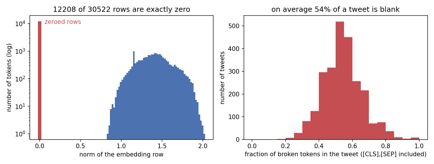
12 208 rows (40 %) are exactly the zero vector, the other 18 314 look perfectly healthy (norms between 0.8 and 2.0). The zeroed rows are spread uniformly over the vocabulary, with no preference for frequent or rare pieces.
The victims include the most important tokens of all: [CLS] and [SEP], which BERT puts at the start and end of every input. The classification head reads the final state of [CLS], so the model now starts every tweet with a blank.
Also broken: ., !, [UNK], [MASK] and thousands of ordinary words. On average 54 % of the tokens of a tweet are blank, and every single tweet is affected.

What does a zero row do? BERT adds the word vector, a position vector and a segment vector, then normalises. With a zero word vector, the token keeps only its position: the network sees "some word was here" and nothing more. Not surprisingly, the broken model scores a macro-F1 of 0.289, below the 0.33 of a constant guess.

The tweets themselves: 935 negative, 806 positive, 759 neutral, 73 characters on average.

A first baseline

The first reflex is to replace every zero row by the mean of the healthy rows. A blank then at least looks like "an average word" instead of an impossible input. Macro-F1 rises to 0.332. Better, but the model still cannot tell "love" from "hate" if one of them is broken.

A smarter guess for a broken token uses the only thing we still know about it: its spelling. Words that share character pieces often have related embeddings (happy, happily, ##ness...). We describe each token by TF-IDF counts of its character 1- to 4-grams (with markers for word start/end and for ## continuation pieces), fit a ridge regression from those features to the 768 coordinates on the 18 314 healthy rows, and predict the broken ones. On held-out healthy rows the prediction is only modestly better than the mean vector (cosine 0.71 against 0.67), but the model's macro-F1 jumps to 0.415.

The key idea

The rest of the network is intact, so it can tell us what the missing vectors should be: treat the broken rows as the only trainable parameters and fit them by gradient descent through the frozen BERT, on the labelled tweets.

Write the repaired matrix as $W = W_{\text{guess}} + M \odot \Delta$ , where $M$ is a 0/1 mask over rows and $\Delta$ the correction we learn. The loss is the usual cross-entropy of the frozen classifier,

\mathcal{L}(\Delta) = -\frac{1}{N}\sum_{i=1}^{N} \log p_\theta\big(y_i \mid \text{tweet}_i ;\ W_{\text{guess}} + M\odot\Delta\big),

and backpropagation flows through all 12 layers down to the embedding rows. This is the right objective because it is exactly the job those rows had during the original fine-tuning: produce vectors that make the frozen layers above output the right sentiment.

The danger is overfitting. There are 12 208 broken rows of 768 numbers each, and only 2 000 training tweets per fold. Two facts guide the choice of $M$ :

A few rows matter enormously. Tuning only [CLS] and [SEP] (1 536 numbers, present in every tweet) lifts the score from 0.398 to 0.479 on an 80/20 split. Each of them gets 2 000 training examples, so they are learned reliably.
Rare rows cannot be learned. A token seen in 2 tweets gets 2 gradient signals and simply memorises those labels. Tuning every broken row gave 0.47 to 0.51 on the same split, depending on the number of epochs; restricting to the broken tokens that appear in at least 20 training tweets (about 120 rows, plus [CLS] and [SEP]) gave the best and most stable result. The rare tokens keep their spelling guess.

So the spelling regression handles the long tail, and the labelled data handles the head of the distribution. The tokens whose vectors moved most during tuning are telling: wish, no, enjoy, feel, better, should, today, (: frequent words that carry sentiment or negation and that no spelling can explain.

The full solution

Locate the damage: rows with norm exactly 0.
Spelling guess: char 1-4-gram TF-IDF of every token, ridge regression ( $\alpha = 3$ ) trained on the healthy rows, predictions written into the broken rows.
Polish by backpropagation: freeze the whole model, make only $\Delta$ trainable on the rows of [CLS], [SEP] and the broken tokens present in at least 20 training tweets. Adam, learning rate $10^{-3}$ , batch 32, 4 epochs, dropout left on as a regulariser.

x = F.embedding(enc["input_ids"], base + mask * delta)   # only masked rows can move
logits = model(inputs_embeds=x, attention_mask=enc["attention_mask"]).logits
loss = F.cross_entropy(logits, labels)

Train once more on all 2 500 labelled tweets and label the test set with the repaired model.

One epoch takes about 25 s on the Apple GPU; the whole 5-fold evaluation runs in about 10 minutes.

Results

approach	macro-F1
broken model (zeros)	0.289
zeros replaced by the mean healthy vector	0.332
spelling guess (char n-gram ridge)	0.415
"context inversion": predict each vector from the hidden states around its position (failed)	0.34 to 0.37
spelling guess + tune `[CLS]`, `[SEP]` only (80/20 split)	0.479
spelling guess + tune all broken rows (80/20 split)	0.47 to 0.51
spelling guess + tune `[CLS]`, `[SEP]` and rows in at least 20 tweets (5-fold CV)	0.561 ± 0.015
same + one round of pseudo-labels on confident test tweets (5-fold CV)	0.563 ± 0.027

Macro-F1 of each repair

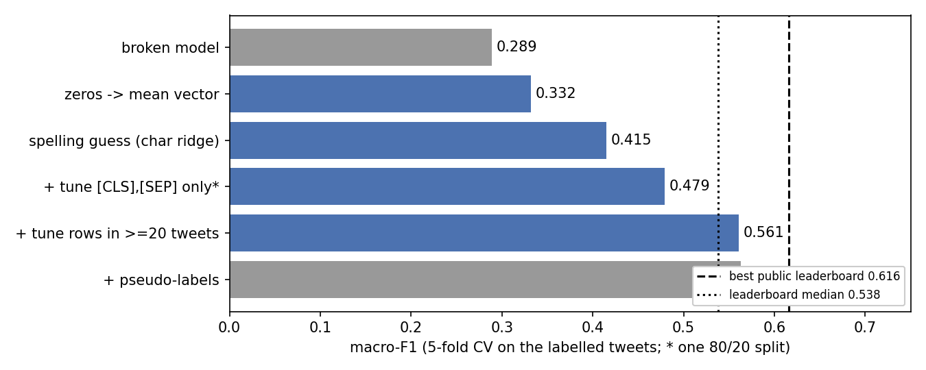
The final repair reaches 0.561 macro-F1 in 5-fold cross-validation, above the leaderboard median (0.538) and below the best public score (0.616). The comparison is indicative only, since the leaderboard is computed on the hidden test tweets.

Two ideas did not pay. Context inversion: BERT was pretrained to guess a hidden word from its context, so the hidden state at a blank position should "know" the missing word; we fitted a ridge map from those states to the true vectors of healthy tokens (blanked on purpose) and applied it to the broken ones. With only 5 000 short tweets, half of whose context is itself blank, the predicted vectors were worse than the spelling guess (centred cosine 0.30 against 0.37 on frequent tokens), and the F1 fell. Pseudo-labelling the confident test tweets and re-tuning gave +0.002, well inside the noise, at twice the cost, so the final solution leaves it out.

What to remember

Diagnose the damage before repairing it. One histogram of row norms showed that the corruption is "exactly zero", which tells you which rows to fix and that the others can be trusted.
Frozen networks are excellent teachers. When part of a model is broken and the rest is intact, make only the broken part trainable and backpropagate the task loss through everything else. The same trick underlies prompt tuning and textual inversion.
Spend your labels where they carry signal. A handful of tokens present in every input ([CLS], [SEP]) give most of the gain; parameters seen in two examples only memorise them. Choosing which parameters to free is a form of regularisation.
Cheap priors cover the long tail. A ridge regression on character n-grams is crude, yet it fills thousands of rare rows with something better than a constant, and it is the right starting point for gradient descent.

"""Broken BERT (Cyprus AI Camp 2026): repair the zeroed rows of a BERT token-embedding matrix.

Data: val_dataset.csv / test.csv from the Kaggle competition, model Ilseyar-kfu/broken_bert (HF),
both in the working folder (model files in ./bb). Test labels are private: we score by 5-fold
cross-validation on the 2 500 labelled validation tweets.

Pipeline
  1. find the broken rows (exactly zero vectors: 12 208 of 30 522, including [CLS] and [SEP]);
  2. fill them with a "spelling" guess: ridge regression from character n-grams of the token
     to its embedding, learned on the 18 314 intact rows;
  3. polish the rows that matter by gradient descent through the frozen network on the labelled
     tweets: [CLS], [SEP] and the broken tokens that occur in at least MIN_COUNT training tweets;
  4. (optional) one round of pseudo-labelling on the confident test tweets.
Usage: python solution.py cv        -> 5-fold CV score
       python solution.py final     -> train on all 2 500 tweets, write submission.csv
"""
import os, sys
os.environ.setdefault("OMP_NUM_THREADS", "2")
import numpy as np, pandas as pd, torch
from sklearn.feature_extraction.text import TfidfVectorizer
from sklearn.linear_model import Ridge
from sklearn.metrics import f1_score
from sklearn.model_selection import StratifiedKFold
from collections import Counter
from transformers import AutoTokenizer, AutoModelForSequenceClassification

torch.set_num_threads(2)
DEV = "mps" if torch.backends.mps.is_available() else "cpu"
MIN_COUNT, EPOCHS, LR, BS = 20, 4, 1e-3, 32
PSEUDO = "--pseudo" in sys.argv
LAB = ["neutral", "positive", "negative"]          # LABEL_0, LABEL_1, LABEL_2 of the model head

tok = AutoTokenizer.from_pretrained("bb")
model = AutoModelForSequenceClassification.from_pretrained("bb").eval()
for p in model.parameters():
    p.requires_grad_(False)
E0 = model.bert.embeddings.word_embeddings.weight.detach().numpy().copy()
val, test = pd.read_csv("val_dataset.csv"), pd.read_csv("test.csv")
y = val.labels.map({l: i for i, l in enumerate(LAB)}).values

# ---------- 1-2. broken rows and the spelling-based first guess ----------
zero = np.linalg.norm(E0, axis=1) == 0
vocab = tok.convert_ids_to_tokens(range(len(E0)))
spell = [("#" + t[2:]) if t.startswith("##") else ("^" + t + "$") for t in vocab]
X = TfidfVectorizer(analyzer="char", ngram_range=(1, 4), min_df=2, sublinear_tf=True).fit_transform(spell)
mu = E0[~zero].mean(0)
ridge = Ridge(alpha=3).fit(X[~zero], E0[~zero] - mu)
E_char = E0.copy()
E_char[zero] = ridge.predict(X[zero]) + mu


def predict_proba(E, texts, bs=64):
    model.to(DEV).eval()
    W = torch.tensor(E, dtype=torch.float32, device=DEV)
    out = []
    with torch.no_grad():
        for i in range(0, len(texts), bs):
            enc = tok(list(texts[i:i + bs]), truncation=True, padding=True, max_length=128,
                      return_tensors="pt").to(DEV)
            x = torch.nn.functional.embedding(enc["input_ids"], W)
            lg = model(inputs_embeds=x, attention_mask=enc["attention_mask"],
                       token_type_ids=enc["token_type_ids"]).logits
            out.append(torch.softmax(lg, -1).cpu().numpy())
    return np.concatenate(out)


# ---------- 3. polish the frequent broken rows on labelled tweets ----------
def polish(E_init, texts, labels, seed=0):
    cnt = Counter(i for t in texts for i in set(tok(t)["input_ids"]))
    sel = np.zeros(len(E0), bool)
    sel[[i for i, c in cnt.items() if c >= MIN_COUNT]] = True
    sel[[tok.cls_token_id, tok.sep_token_id]] = True
    sel &= zero                                      # only broken rows may move
    model.to(DEV).train()                            # dropout on: a cheap regulariser
    base = torch.tensor(E_init, dtype=torch.float32, device=DEV)
    mask = torch.tensor(sel, device=DEV)[:, None].float()
    delta = torch.zeros_like(base, requires_grad=True)
    opt = torch.optim.Adam([delta], lr=LR)
    yt = torch.tensor(labels)
    g = torch.Generator().manual_seed(seed)
    for ep in range(EPOCHS):
        perm = torch.randperm(len(texts), generator=g).numpy()
        for i in range(0, len(perm), BS):
            b = perm[i:i + BS]
            enc = tok(list(texts[b]), truncation=True, padding=True, max_length=128,
                      return_tensors="pt").to(DEV)
            x = torch.nn.functional.embedding(enc["input_ids"], base + mask * delta)
            lg = model(inputs_embeds=x, attention_mask=enc["attention_mask"],
                       token_type_ids=enc["token_type_ids"]).logits
            loss = torch.nn.functional.cross_entropy(lg, yt[b].to(DEV))
            opt.zero_grad(); loss.backward(); opt.step()
    return (base + mask * delta).detach().cpu().numpy()


def fit(texts, labels, unlabelled):
    E = polish(E_char, texts, labels)
    if PSEUDO:                                       # 4. one round of self-training
        p = predict_proba(E, unlabelled)
        keep = p.max(1) > 0.8
        E = polish(E_char, np.concatenate([texts, unlabelled[keep]]),
                   np.concatenate([labels, p.argmax(1)[keep]]))
    return E


if __name__ == "__main__":
    mode = sys.argv[1] if len(sys.argv) > 1 else "cv"
    texts = val.text.values
    if mode == "cv":
        scores = {"broken": [], "char fill": [], "polished": []}
        for k, (tr, ho) in enumerate(StratifiedKFold(5, shuffle=True, random_state=0).split(texts, y)):
            for name, E in [("broken", E0), ("char fill", E_char),
                            ("polished", fit(texts[tr], y[tr], test.text.values))]:
                if name == "broken" and k > 0:
                    continue
                s = f1_score(y[ho], predict_proba(E, texts[ho]).argmax(1), average="macro")
                scores[name].append(s)
            print(k, {n: round(v[-1], 4) for n, v in scores.items()}, flush=True)
        print({n: (round(np.mean(v), 4), round(np.std(v), 4)) for n, v in scores.items()})
    else:
        E = fit(texts, y, test.text.values)
        np.save("E_final.npy", E)
        pred = predict_proba(E, test.text.values).argmax(1)
        pd.DataFrame({"labels": [LAB[i] for i in pred], "id": test.id}).to_csv("submission.csv", index=False)
        print("wrote submission.csv", pd.Series([LAB[i] for i in pred]).value_counts().to_dict())