Trace Twins

The problem in brief

A malware analyst records, for each suspicious program run in a sandbox, the sequence of system calls it makes (about 270 possible commands such as ntopenkey or ldrloaddll). Each recording is cut into windows of exactly 200 calls. You must write a function that receives pairs of windows and returns a score that is higher when the two windows were cut from the same program. The negatives are nasty: every "different program" pair is drawn from the same malware category (two Trojans, two Worms...), so you cannot win by recognising the category. In Part A the command names are real; in Part B every window has been renamed with its own random permutation of the vocabulary, so the same call has a different name in each window. You submit a pickled Python object; it is run on programs never seen in training.

How you are scored

Each part is scored by the ROC-AUC of your scores over 3,000 pairs (half twins, half same-category strangers):

$$\text{AUC} = P\big(s(\text{twin pair}) > s(\text{stranger pair})\big),$$

the probability that a random positive pair is ranked above a random negative pair (0.5 = coin flip). It is then turned into points:

$$\text{Part A} = \operatorname{round}\Big(\max\big(3, \min(50,\ 3 + 47\,\tfrac{A_A - 0.5}{0.34})\big)\Big),\qquad \text{Part B} = \operatorname{round}\Big(\max\big(2, \min(50,\ 2 + 48\,\tfrac{A_B - 0.5}{0.28})\big)\Big).$$

So the targets are AUC 0.84 in Part A and 0.78 in Part B, each worth the full 50 points (statement, "Scoring" section).

How we evaluate. The round's test_data.csv contains the test programs with their program_id, and the organisers published the pre-judging script with its seeds (program split, pair sampling, scrambling). Re-running that exact construction gives the official 3,000 + 3,000 test pairs with their labels. We never looked at these pairs while developing: all choices were made on a validation split of the training programs (30 % of programs held out, as in the starter notebook).

First look at the data

The training file has 4,843 programs in 8 categories, with traces of 100 to 4,000 calls (median about 800), so a program contributes between 0 and 8 windows. Three observations guide everything:

• Traces are extremely repetitive. Many windows are long loops of two or three calls (ldrgetprocedureaddress repeated 200 times is common). Two different programs that both spend a window in such a loop look identical, which caps what any method can reach.
• Twins share a vocabulary, not a position. Two windows of the same program can be far apart in time, so they rarely share long exact substrings, but they tend to use the same set of calls in similar proportions.
• In Part B the names are not random strings, they are other real names. The renaming is a permutation of the vocabulary, so a scrambled window "looks" like a normal one but every name lies.

A first baseline

Part A. Treat each window as a document whose "words" are its calls and its 2- and 3-grams, weight them by TF-IDF with a logarithmic term frequency, and score a pair by the cosine similarity of the two vectors. Validation AUC: 0.80 (0.785 on the official test), which gives 43 points. It is a fair baseline: no learning at all, just "do they use the same words?".

Part B. That baseline is useless after renaming: the same call has a different name in each window, so any feature that uses names scores AUC 0.5 (2 points).

The key idea

There are two ideas, one per part.

Part A: learn what "similar" means instead of fixing it. Cosine similarity treats every shared call as equal evidence. But sharing ntclose (used by every program) means little, while sharing a rare registry call in similar proportions means a lot, and "similar proportions" itself depends on the call. So we turn the pair problem into an ordinary classification problem. For a pair $(u, v)$ with frequency vectors $f_u, f_v \in \mathbb{R}^{270}$ we build symmetric pair features

$$\phi(u, v) = \big[\min(f_u, f_v),\ |f_u - f_v|,\ \cos(u,v),\ \text{Jaccard}(u,v),\ \min(d_u, d_v),\ |d_u - d_v|\big]$$

($d$ = number of distinct calls), and train gradient-boosted trees on tens of thousands of labelled pairs sampled from the training programs exactly as the grader samples them (half twins, half same-category strangers). The model learns which calls are discriminative and how much disagreement is normal. Symmetry matters: $\phi(u,v) = \phi(v,u)$, so the score cannot depend on the order of the pair.

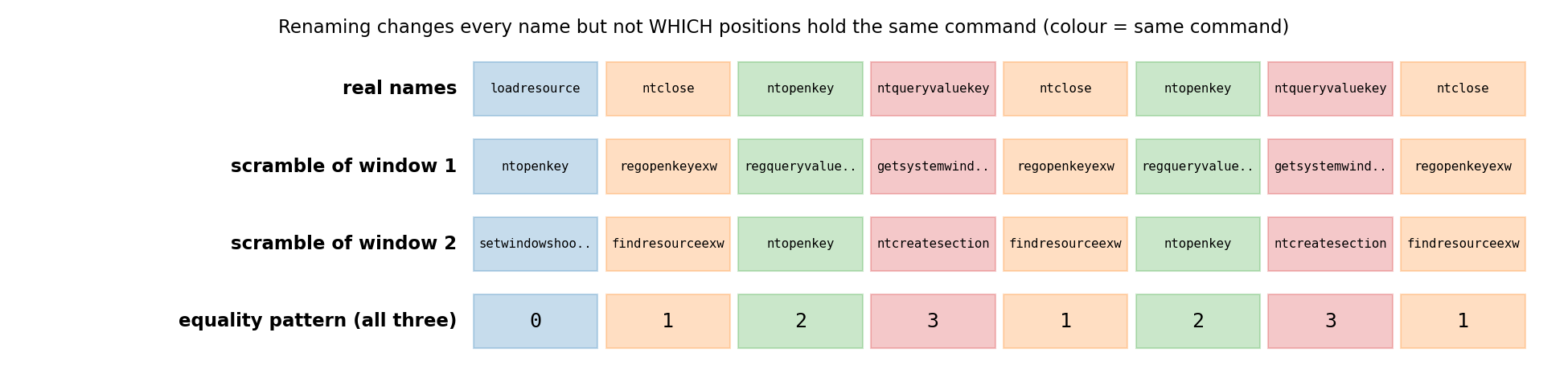
Part B: describe each window with what a renaming cannot change. If $\pi$ is the secret permutation of a window, any statistic $T$ with $T(\pi(w)) = T(w)$ for every $\pi$ survives the scrambling. Three families of such invariants:

1. Equality patterns. Replace each short $n$-gram by the pattern of which positions are equal: ntclose ntopenkey ntclose and abc xyz abc both become 0 1 0. These patterns describe the control flow of the program (loops, alternations, open/query/close rhythms).
2. Frequency ranks. Rename every call by its rank of frequency within the window (0 = most frequent). The relabelled sequence is identical whatever the renaming, as long as the window keeps the same frequency profile.
3. Recurrence gaps. For each call, the distance since its previous occurrence (log-binned). A loop of period 3 produces gaps of 3, whatever the names.

Each family becomes a bag of "words" (p5:01201, r2:0,3, g:4...), and each gives a TF-IDF cosine between the two windows. Then we reuse the Part A recipe: boosting on these nine cosines plus symmetric summaries of the frequency profile (sorted counts, entropy, number of runs). To make the training pairs look like the test pairs, we scramble the training windows with the organisers' own scrambling function.

Why does this not destroy the information? Because what identifies a program is not the spelling of its calls but its behaviour: the same loops, the same call rhythms, the same balance between a few dominant calls. All of that is invariant.

The full solution

1. Windows and pairs. Cut the training traces into windows with the organisers' code, then sample 40,000 labelled pairs per part with the grader's sampling rule (same-category negatives).

2. Part A features. Frequency vectors over the 270 calls, TF-IDF on 1- to 3-grams (fitted on training windows only), cosine and Jaccard similarity, distinct-call counts, combined symmetrically.

3. Part B features. Scramble the training windows; build the invariant words; one TF-IDF model per family; nine cosines plus profile summaries.

   def canon(seq):                      # ("ntclose","ntopenkey","ntclose") -> (0, 1, 0)
       m = {}; return tuple(m.setdefault(t, len(m)) for t in seq)
   words += [f"p{n}:" + "".join(map(str, canon(w[i:i+n]))) for n in (3,4,5,6)
             for i in range(len(w) - n + 1)]
   

4. Models. One HistGradientBoostingClassifier per part (300 trees, learning rate 0.08); the score of a pair is the predicted probability of "twin".

5. Submission. Everything (vectorisers and models) lives inside the Submission object, which implements score_A, score_B and the __call__ protocol of the grader, so cloudpickle captures a self-contained file. Training takes about 3 minutes on 2 CPU threads.

Results

approach	Part A AUC	Part B AUC	points
constant score (starter notebook)	0.500	0.500	3 + 2 = 5
Jaccard of call sets (validation)	0.750	0.5 (names useless)	38 + 2
TF-IDF 1-3-gram cosine (validation)	0.804	0.5	45 + 2
same, official test	0.785		42
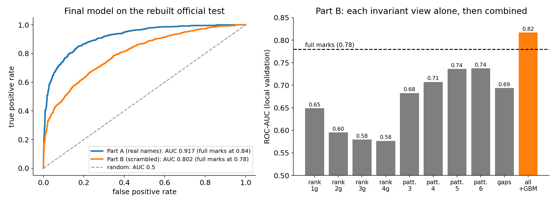
Part B: best single invariant view, 6-gram equality patterns (validation)		0.737	43
Part B: recurrence gaps + profile, boosted (validation; first try with a bug that silently disabled the other views)		0.785	50
pairwise boosting, all features (validation)	0.917	0.817	50 + 50
final model, rebuilt official test	0.917	0.802	50 + 50 = 100

Two lessons hide in this table. First, learning the similarity is worth more than any hand-tuning of the cosine: the jump from 0.80 to 0.92 in Part A comes only from letting a model weigh the evidence. Second, no single invariant view reaches the Part B target, but they are complementary: equality patterns see the control flow, ranks see the frequency profile, gaps see the loop periods, and the combination clears 0.78 comfortably.

The "bug" row is a classic Python trap worth knowing: building several TfidfVectorizer(analyzer=lambda d: ... pre ...) in a loop makes every lambda use the last value of pre, so all views silently became the same one (their AUCs were all exactly 0.5 except the last). Binding the loop variable with lambda d, pre=pre: ... fixes it.

What to remember

• A pair-scoring task is a classification task on pairs. Build symmetric pair features ($\min$, $|\,\cdot - \cdot\,|$, similarities) and train on pairs sampled like the grader samples them, including the hard negatives.
• When the input is corrupted by a group of transformations, look for invariants. Here the group is "all renamings", and equality patterns, frequency ranks and recurrence distances are invariant to it. The same reflex works for images (rotation-invariant features), sets (order-invariant pooling) and graphs.
• Make the training data suffer the same corruption as the test data. Scrambling the training windows with the organisers' function is what lets the model learn which invariants matter.
• Combine weak complementary views. Several 0.6 to 0.74 signals that see different aspects of the data beat any single one.
• Rebuild the grader locally whenever its code is public. It turns guesswork into an exact score, and it catches format errors before they cost a submission.