IOAI Training: Learn AI by solving problems

The problem in brief

A plain but large binary classification: one million training rows, 285 anonymous features, and a 0/1 target to predict as a probability for the test rows. The competition page reuses the text and data of Kaggle's Tabular Playground Series of October 2021: the data are synthetic, generated by a GAN (CTGAN) trained on a real dataset about the biological response of molecules. 240 features are continuous values in $[0, 1]$ , 45 are binary, and there are no missing values. There is nothing to read into the column names, so the problem is about method: handle the size, find what carries the signal, and regularise.

The data are the official Kaggle files. The test labels are private and we did not submit anything. Because the training file is 2.3 GB and our machine allows 3 GB of memory per process, we kept the first 400 000 training rows: 300 000 to train, 100 000 held out for every score below.

How you are scored

ROC AUC of the predicted probabilities: the probability that a random positive row gets a higher score than a random negative row,

\text{AUC} = \Pr\big(\hat p(x^+) > \hat p(x^-)\big).

Only the ranking matters. A constant prediction scores 0.5 and a perfect ranking 1.

What to aim for. No threshold is published. On the public leaderboard the best entry has 0.8551, and the top eight all lie between 0.848 and 0.855.

First look at the data

The target is balanced: 51.2 % positives.
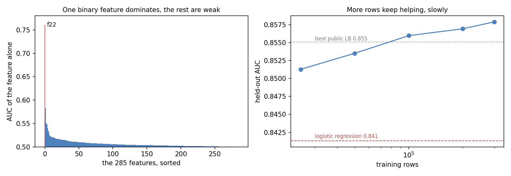
Taken one at a time, almost every feature is useless: all but a handful of the 285 single-feature AUCs are below 0.55. One feature stands out completely: the binary f22. When f22 = 0, 79 % of rows are positive; when f22 = 1, only 27.5 % are. On its own it gives AUC 0.761 (left panel). The next best feature, f179, gives 0.58.

Single-feature AUCs and learning curve

Memory matters. Read naively with pandas, the 1 million × 287 table takes about 2.3 GB in float64, before any model is built. We read the file in chunks of 50 000 rows, convert each chunk to float32, and stop at 400 000 rows (456 MB).

A first baseline

Logistic regression on 100 000 rows (with $C = 0.1$ ): AUC 0.841. It is already far above f22 alone, so the many weak features do add up. Gradient boosting with LightGBM's defaults (31 leaves, learning rate 0.1) on 300 000 rows: 0.856.

The key idea

Many weak, noisy signals call for many small, heavily regularised trees. Removing f22 drops a tuned model from 0.858 to 0.695: f22 is worth more than everything else combined. Everything beyond f22 comes from a few hundred features that each move the odds a tiny bit. That has three consequences for the model:

Small trees. With weak effects, deep trees mostly fit noise. We use 15 leaves per tree and a low learning rate (0.03), so the model is a long sum of small corrections (about 2 000 trees, chosen by early stopping on the held-out rows).
Column subsampling. Each tree sees a random 15 % of the columns (feature_fraction = 0.15). Otherwise, after f22, every tree would pick the same few strong columns and ignore the hundreds of weak ones. Forcing variety spreads the work over all features, which is what helps when the signal is spread out.
Strong regularisation. At least 200 rows per leaf and an L2 penalty of 10 on leaf values keep each leaf's estimate stable. GAN-generated data contain many spurious patterns that a flexible model would happily memorise.

The learning curve (right panel) shows the other lever: more data keeps helping. The tuned model scores 0.851 with 25 000 rows, 0.856 with 100 000, and 0.858 with 300 000. Each doubling buys less, but it still buys something, so training on the full million rows (on a machine with more memory) would be worth a little more.

The full solution

Stream the first 400 000 rows of train.csv into a float32 array.
Split: the first 300 000 rows to train, the last 100 000 to validate. The data are synthetic rows with no time structure, so a contiguous split behaves like a random one.
Train LightGBM:

params = dict(objective="binary", metric="auc", learning_rate=0.03, num_leaves=15,
              feature_fraction=0.15, min_child_samples=200, lambda_l2=10, max_bin=63,
              num_threads=2)
model = lgb.train(params, dtr, 4000, valid_sets=[dva],
                  callbacks=[lgb.early_stopping(100)])

Predict the test file in chunks of 50 000 rows (if it has been downloaded; we did not need it, since we did not submit).

Results

All scores are AUC on the same 100 000 held-out training rows. The official test labels are private.

approach	held-out AUC
f22 alone	0.761
tuned LightGBM without f22	0.695
logistic regression, 100 000 rows	0.841
LightGBM, default settings, 300 000 rows	0.856
tuned LightGBM, 25 000 / 50 000 / 100 000 / 200 000 rows	0.851 / 0.854 / 0.856 / 0.857
tuned LightGBM, 300 000 rows (final)	0.858

Our final held-out AUC of 0.858 is slightly above the best public leaderboard score (0.855). The two numbers are not measured on the same rows, but with 100 000 held-out rows the standard error of our AUC is only about 0.001, so the comparison suggests that our pipeline is at the level of the top entries. One caveat: early stopping picked the number of trees on these same held-out rows, which flatters the score slightly; with 100 000 rows and a single tuned quantity the effect is small.

What to remember

Check single-feature AUCs first. It takes seconds and here it found the one feature (f22) that carries most of the signal.
When the signal is spread over many weak features, make each tree small and let it see few columns. Low learning rate, few leaves, column subsampling and leaf regularisation beat a default model.
Measure what a feature is worth by removing it. Without f22 the model loses 0.16 of AUC; importance scores (60 % of the gain) say the same in a less direct way.
Big files do not need big memory. Read in chunks, convert to float32, keep what you need. A learning curve then tells you whether more rows would actually help.
Early stopping on a held-out set chooses the number of trees for you. Use a set you will not tune anything else on if you want an honest final number.

"""Benin national AI olympiad selection 2025 (Kaggle): binary classification on synthetic tabular data.

The data are the Kaggle Tabular Playground Series of October 2021 (CTGAN-generated from a molecular
biological-response dataset): 1 000 000 training rows, 285 anonymous features (240 continuous in
[0, 1], 45 binary), ROC AUC. The train file is 2.3 GB, so we stream it and keep the first 400 000
rows as float32 (456 MB): 300 000 to train, 100 000 held out. Official test labels are private.

Findings: one binary feature, f22, carries most of the signal (target rate 79 % vs 27 %, AUC 0.76
alone; without it a tuned model falls to 0.695). The rest is many weak features: gradient boosting
with small trees, strong column subsampling and regularisation reaches 0.858 on the held-out rows.

Usage: python solution.py [folder with train.csv (and optionally test.csv)]
"""
import os
import sys
import numpy as np
import pandas as pd
import lightgbm as lgb
from sklearn.linear_model import LogisticRegression
from sklearn.metrics import roc_auc_score

D = sys.argv[1] if len(sys.argv) > 1 else "work"
N_KEEP, N_TRAIN = 400_000, 300_000


def load_rows(path, n):
    """Read the first n rows in chunks of 50 000, as float32 (pandas would use ~3x more memory)."""
    parts, got = [], 0
    for ch in pd.read_csv(path, chunksize=50_000):
        parts.append(ch.astype("float32"))
        got += len(ch)
        if got >= n:
            break
    return pd.concat(parts).iloc[:n]


df = load_rows(f"{D}/train.csv", N_KEEP)
feats = [c for c in df.columns if c not in ("id", "target")]
X, y = df[feats].values, df.target.values.astype(int)
del df
Xa, ya, Xv, yv = X[:N_TRAIN], y[:N_TRAIN], X[N_TRAIN:], y[N_TRAIN:]

# ---------------------------------------------------------------- 1. look at single features
j22 = feats.index("f22")
print(f"f22 = 0: {ya[Xa[:, j22] == 0].mean():.1%} positives, f22 = 1: {ya[Xa[:, j22] == 1].mean():.1%}")
print(f"AUC of f22 alone: {1 - roc_auc_score(yv, Xv[:, j22]):.4f}")

# ---------------------------------------------------------------- 2. baseline
lr = LogisticRegression(max_iter=300, C=0.1).fit(Xa[:100_000], ya[:100_000])
print(f"logistic regression (100k rows): AUC {roc_auc_score(yv, lr.predict_proba(Xv)[:, 1]):.4f}")

# ---------------------------------------------------------------- 3. gradient boosting
params = dict(objective="binary", metric="auc", verbose=-1, num_threads=2,
              learning_rate=0.03, num_leaves=15,      # small trees: many weak, additive effects
              feature_fraction=0.15,                  # each tree sees 15 % of the 285 columns
              min_child_samples=200, lambda_l2=10,    # strong regularisation against GAN noise
              max_bin=63)
dtr = lgb.Dataset(Xa, ya)
dva = lgb.Dataset(Xv, yv, reference=dtr)
model = lgb.train(params, dtr, 4000, valid_sets=[dva], callbacks=[lgb.early_stopping(100, verbose=False)])
p = model.predict(Xv, num_iteration=model.best_iteration)
print(f"LightGBM, {model.best_iteration} trees: held-out AUC {roc_auc_score(yv, p):.4f}")
gain = model.feature_importance("gain")
print("largest gain shares:", [(feats[j], round(gain[j] / gain.sum(), 3)) for j in np.argsort(-gain)[:5]])

# ---------------------------------------------------------------- 4. optional test predictions
if os.path.exists(f"{D}/test.csv"):
    out = []
    for ch in pd.read_csv(f"{D}/test.csv", chunksize=50_000):
        out.append(pd.DataFrame({"id": ch.id, "target": model.predict(ch[feats].values.astype("float32"),
                                                                       num_iteration=model.best_iteration)}))
    pd.concat(out).to_csv("submission.csv", index=False)
    print("wrote submission.csv (not submitted)")

Binary Classification on Synthetic Tabular Data