IOAI Training: Learn AI by solving problems

The problem in brief

Each row describes one wild blueberry field during flowering: the size of the plant clones, the density of four kinds of bees (honeybees, bumblebees, Andrena and Osmia), six temperature statistics, two rain statistics, and three measurements of the result (the fraction of flowers that became fruit, the mean fruit mass and the mean number of seeds per berry). You must predict the yield for 195 test fields after training on 582. The starter notebook suggests kNN, gradient boosting and a small neural network, with deliberately poor settings, and asks you to choose features and tune a model.

The task files come from a personal GitHub mirror of the round (github.com/yonitoo/awesome-BGOAI-tasks), and the test file has no yields. But the 777 rows are exactly the public Wild Blueberry Pollination Simulation dataset (Obsie, Qu and Drummond, 2020), and every test row matches exactly one row of the public file on its three fruit measurements. We therefore recovered the test labels from the public original dataset, made every choice by cross-validation on the training set, and scored the test set once at the end.

How you are scored

The metric is the mean absolute error:

\text{MAE} = \frac{1}{n}\sum_{i=1}^{n} \lvert \hat{y}_i - y_i \rvert .

Lower is better. Two consequences matter. First, MAE is minimised by the median of the conditional distribution, not the mean, so it is natural to train with an absolute loss too. Second, MAE is linear in the size of each error, so a few rare rows with large errors do not dominate it as much as they would dominate RMSE.

The statement publishes no threshold and we found no leaderboard. As reference points: always predicting the median yield gives a test MAE of 1 070, and yields range from about 1 600 to 9 000.

First look at the data

The 16 columns are not 16 pieces of information. Counting distinct values tells the real story:

The six temperature columns take only 5 distinct combinations: each field got one of 5 temperature profiles, and the six numbers are fully determined by the profile. The two rain columns likewise take 5 combinations.
Clone size and the four bee densities each take a handful of values (6 to 11).
Only fruitset, fruitmass and seeds are continuous, with a different value in every row.

This is the fingerprint of a computer simulation. The researchers ran a model of pollination on a grid of scenarios (7 "knobs": clone size, 4 bee densities, temperature profile, rain profile), each row being the average of 100 simulation runs. The three fruit measurements are outputs of the same simulation as the yield. So we keep one column per knob (MaxOfUpperTRange stands for the temperature profile, RainingDays for the rain profile) and the three outputs.

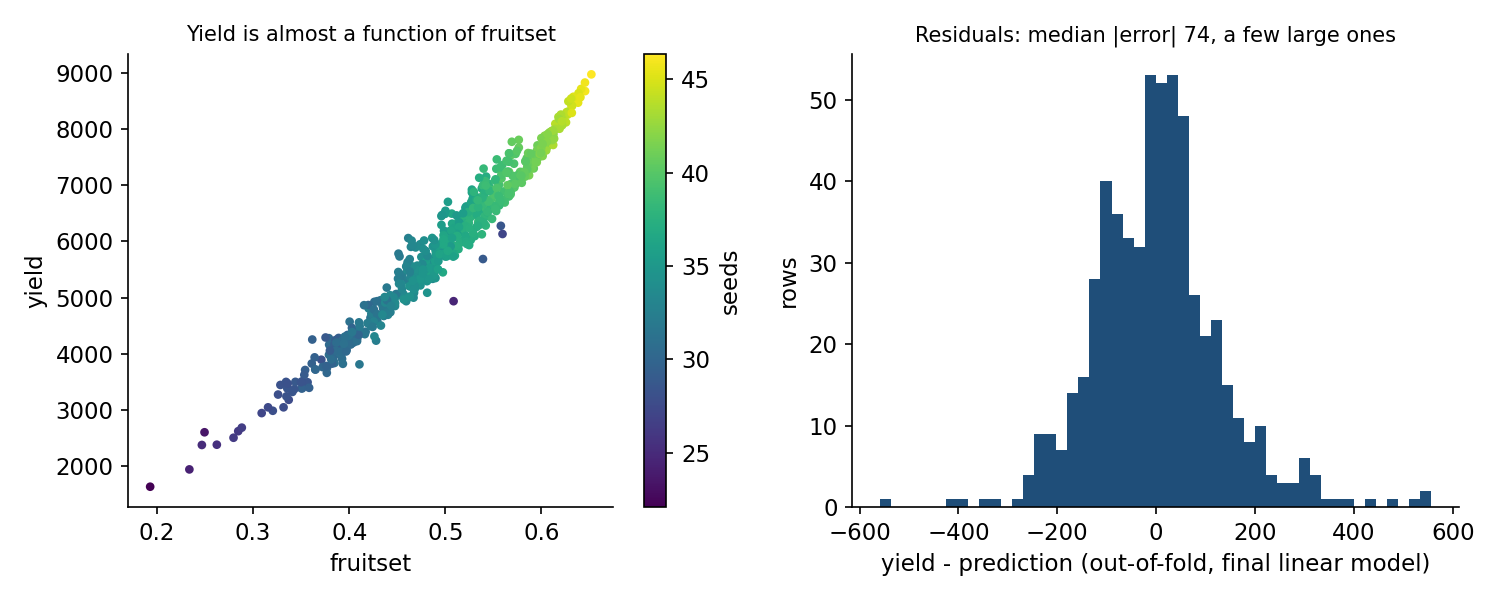
Yield against fruitset, and residuals of the final model

Yield is almost a function of fruitset (correlation 0.984, left panel), with seeds (0.960) and fruitmass (0.929) close behind. A model is not needed to discover that yield comes from fruit: it is needed to squeeze out the remaining 2 % of variance. The relation also looks slightly curved and multiplicative: the spread grows with the yield, which hints at working in logarithms.

A few rows are off the grid. Most fields have clone size 12.5, 25 or 37.5 and honeybee density 0.25, 0.5 or 0.75. But 14 training rows (2.4 %) are special scenarios: clone size 20, honeybee densities of 6.64 or 18.43, a rain profile of 3.77 days that appears nowhere else. They will turn out to be where the large errors live.

A first baseline

The starter models are deliberately weak, and each one teaches something:

starter model	CV MAE	why it is weak
gradient boosting, 5 trees of depth 10	675	5 trees with the default learning rate of 0.1 cover only about 40 % of the way from the mean to the target ( $1 - 0.9^5 \approx 0.41$ )
kNN, $k = 3$ , all 16 columns scaled	218	in the distance, the 13 design columns (most of them copies of the same knob) outnumber the 3 informative outputs 13 to 3
MLP 64-64	164	needs far more than 582 rows to learn a nearly linear relation

A plain linear regression on the three outputs already gets a CV MAE of 136, and adding the design knobs brings it to about 103. Simple beats clever here, and the reason is the next section.

The key idea

The target is a simulated quantity built multiplicatively from the other simulated quantities, so the right model is linear in logarithms, fitted with the loss you are scored on.

Agronomically, yield is (number of flowers) × (fraction that set fruit) × (mass per fruit). Products become sums after taking logs:

\log y \approx \beta_0 + \beta_1 \log(\text{fruitset}) + \beta_2 \log(\text{fruitmass}) + \beta_3 \log(\text{seeds}) + \sum_k \gamma_k\, d_k ,

where the $d_k$ are the 7 design knobs. This model has 11 parameters, so 582 rows are plenty, and it extrapolates sensibly to the edges of the data, where trees cannot.

Fit it with an absolute loss. sklearn's QuantileRegressor(quantile=0.5) minimises $\sum_i \lvert \log y_i - \hat{f}(x_i) \rvert$ , the median regression. The median of $\log y$ is the log of the median of $y$ (the logarithm is monotonic), so exponentiating its predictions gives a conditional median, exactly what MAE rewards. A least-squares fit would chase the mean and be pulled by the off-grid rows.

What the fitted model says is instructive:

term	coefficient
$\log$ fruitset	+1.14
$\log$ seeds	+1.08
$\log$ fruitmass	−1.08
bees (per unit of density): osmia, andrena, bumbles, honeybee	+0.077, +0.053, +0.042, +0.003
temperature (per °F of the profile's maximum), rain (per rainy day)	−0.0012, −0.0016
clone size	0

The coefficient of fruitset is close to 1, as the multiplicative story predicts: 10 % more fruit set means about 11 % more yield. The seeds and fruitmass coefficients are a warning, not an insight: $\log$ seeds and $\log$ fruitmass are correlated at 0.991, so the model can only estimate their difference, and it ends up using the seeds-per-milligram ratio. With such collinear inputs, never read individual coefficients as causal effects. Note also how small the design terms are once the fruit measurements are known: going from the coolest to the hottest temperature profile changes the prediction by only about 3 %, from the driest to the wettest by about 5 %, and the full range of Osmia density by about 6 %. Most of the effect of weather and bees on yield goes through fruit set, which is what a simulation of pollination should produce; the knobs only correct the remainder.

The full solution

Recover the test labels by matching the test rows to the public original on (fruitset, fruitmass, seeds), and check that the same matching reproduces every training yield exactly. Put them aside.
Reduce the columns to 3 outputs + 7 design knobs, and take logs of the outputs and of the target.
Model A: median regression (L1 loss) of $\log y$ on these 10 features, standardised. CV MAE 95.8.
Model B: gradient boosting with the Huber loss, 600 trees of depth 3, learning rate 0.03, subsampling 0.8, on all columns. CV MAE 102.6. Trees capture the interactions and plateaus that the linear model misses, but extrapolate badly.
Blend: $0.7 \times A + 0.3 \times B$ , the weight chosen by CV (0.5 and 0.7 are tied at 92.4 and 92.3). The two models make different kinds of mistakes (smooth global fit against local, piecewise constant fit), so averaging them helps.

L1 = QuantileRegressor(quantile=0.5, alpha=0.0, solver="highs")   # minimises absolute error
model_A = make_pipeline(StandardScaler(), L1).fit(logfeats(train), np.log(y))
pred = 0.7 * np.exp(model_A.predict(logfeats(test))) + 0.3 * model_B.predict(test)

Where the errors are. The residuals (right panel of the figure above) have a median absolute value of 74 but a few reach 550. Grouping them shows why: the mean absolute residual is about 100 on the regular grid, but 241 for the clone size 20 rows, 228 for the 3.77-day rain profile, and 555 for the honeybee density of 18.43. Those scenarios appear only 1 to 13 times in training, so no model can learn them well. That is the irreducible part of this dataset.

Results

approach	CV MAE (582 train rows)	test MAE (195 rows)
always predict the median	1 116	1 070
starter GBR, 5 trees of depth 10	675	648
starter kNN, $k = 3$	218	191
starter MLP 64-64	164	114
linear regression, all 16 columns	151	93
linear regression, 3 outputs only	136	139
L1 linear, outputs + design	104	95
tuned GBR (Huber loss), all columns	103	93
L1 log-log linear, outputs + design	96	93
blend 0.5 log-log + 0.5 GBR	92.4	87.4
final: blend 0.7 log-log + 0.3 GBR	92.3	87.8

CV and test MAE of each approach

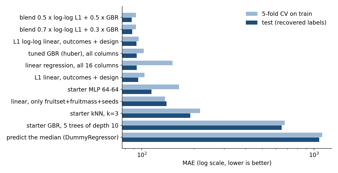
The final model reaches a test MAE of 87.8, about 1.6 % of the mean yield, against 1 070 for the constant baseline.

A lesson in the test column. With only 195 test rows, the test MAE is noisy. Plain linear regression on all 16 columns scores 151 in CV but 93 on test, as well as the tuned models: on this particular test draw it was lucky. A single test score cannot separate models within about 10 MAE of each other here, while the 5-fold CV over 582 rows is a more stable guide. That is why every choice above was made on CV, and why you should never choose a model because of one small test set (or one public leaderboard).

What to remember

Count the distinct values of every column. Six temperature columns with 5 combinations are one variable. Spotting a designed grid tells you how the data was made, which features are redundant and which rows are rare.
Multiplicative processes call for logarithms. When the target is a product of factors (yield = flowers × fruit set × mass), a linear model on logs is small, robust and extrapolates where trees cannot.
Train with the loss you are scored on. MAE rewards the conditional median: fit with an absolute (or Huber) loss, not least squares.
Collinear inputs make coefficients meaningless one by one. With a correlation of 0.991 between log seeds and log fruitmass, only their combination is identified.
Small test sets are noisy. Choose with cross-validation, and treat test differences of a few percent as noise.

"""
Bulgaria NCAI 2026 final, Task 1: wild blueberry yield regression, metric MAE.

Data: train.csv / test.csv from github.com/yonitoo/awesome-BGOAI-tasks (2026/NCAI/R2/Task_1).
The rows are the public "Wild blueberry pollination simulation" dataset (777 rows, Obsie et al. 2020;
copy used: raw.githubusercontent.com/sadiaanzum/Wild-Blueberry-Yield-Prediction/master/
WildBlueberryPollinationSimulationData.csv, saved as orig.csv). Every test row matches exactly one
original row on (fruitset, fruitmass, seeds), which recovers the test labels.
Model choices use 5-fold CV on train only; the recovered test labels are used once, at the end.

Run: python solution.py   (about 1 minute on CPU; figures go to ./figures)
"""
import os, warnings
import numpy as np, pandas as pd
import matplotlib; matplotlib.use("Agg")
import matplotlib.pyplot as plt
from sklearn.model_selection import KFold, cross_val_predict
from sklearn.pipeline import make_pipeline
from sklearn.preprocessing import StandardScaler
from sklearn.dummy import DummyRegressor
from sklearn.neighbors import KNeighborsRegressor
from sklearn.neural_network import MLPRegressor
from sklearn.linear_model import LinearRegression, QuantileRegressor
from sklearn.ensemble import GradientBoostingRegressor
warnings.filterwarnings("ignore")
DATA_DIR = os.environ.get("DATA_DIR", "work")
FIG = "figures"; os.makedirs(FIG, exist_ok=True)
plt.rcParams.update({"font.size": 11, "axes.spines.top": False, "axes.spines.right": False})

train = pd.read_csv(f"{DATA_DIR}/train.csv", index_col=0)
test = pd.read_csv(f"{DATA_DIR}/test.csv", index_col=0)
orig = pd.read_csv(f"{DATA_DIR}/orig.csv")
y = train.pop("yield")

# ---------------------------------------------------------------- recover test labels from the public original
key = lambda d: d[["fruitset", "fruitmass", "seeds"]].round(6).astype(str).agg("|".join, axis=1)
lab = dict(zip(key(orig), orig["yield"]))
y_test = key(test).map(lab)
assert y_test.notna().all() and key(train).map(lab).sub(y).abs().max() < 1e-6
print("test labels recovered for", len(y_test), "rows")

# ---------------------------------------------------------------- the 16 columns are really 7 design knobs + 3 outcomes
T = ["MaxOfUpperTRange", "MinOfUpperTRange", "AverageOfUpperTRange",
     "MaxOfLowerTRange", "MinOfLowerTRange", "AverageOfLowerTRange"]
print("distinct temperature profiles:", len(train[T].drop_duplicates()),
      "| distinct rain profiles:", len(train[["RainingDays", "AverageRainingDays"]].drop_duplicates()))
DESIGN = ["clonesize", "honeybee", "bumbles", "andrena", "osmia", "MaxOfUpperTRange", "RainingDays"]
OUT = ["fruitset", "fruitmass", "seeds"]
print(train[OUT].corrwith(y).round(3).to_dict())

def logfeats(d):
    """log of the 3 simulated outcomes + the 7 design knobs as they are"""
    L = pd.DataFrame({f"log_{c}": np.log(d[c]) for c in OUT}, index=d.index)
    L[DESIGN] = d[DESIGN]
    return L

# ---------------------------------------------------------------- models
L1 = lambda: QuantileRegressor(quantile=0.5, alpha=0.0, solver="highs")   # minimises absolute error
gbr = lambda: GradientBoostingRegressor(loss="huber", n_estimators=600, learning_rate=0.03,
                                        max_depth=3, subsample=0.8, random_state=0)
ALL = list(train.columns)
models = {  # name: (model, feature function, fit on log(yield)?)
    "predict the median (DummyRegressor)": (DummyRegressor(strategy="median"), lambda d: d, False),
    "starter kNN, k=3": (make_pipeline(StandardScaler(), KNeighborsRegressor(3)), lambda d: d, False),
    "starter MLP 64-64": (make_pipeline(StandardScaler(), MLPRegressor(hidden_layer_sizes=(64, 64),
                          max_iter=3000, random_state=42)), lambda d: d, False),
    "starter GBR, 5 trees of depth 10": (GradientBoostingRegressor(n_estimators=5, max_depth=10,
                                         random_state=42), lambda d: d, False),
    "linear regression, all 16 columns": (LinearRegression(), lambda d: d, False),
    "linear, only fruitset+fruitmass+seeds": (LinearRegression(), lambda d: d[OUT], False),
    "tuned GBR (huber), all columns": (gbr(), lambda d: d, False),
    "L1 linear, outcomes + design": (make_pipeline(StandardScaler(), L1()), lambda d: d[OUT + DESIGN], False),
    "L1 log-log linear, outcomes + design": (make_pipeline(StandardScaler(), L1()), logfeats, True),
}
kf = KFold(5, shuffle=True, random_state=0)
rows, oof, test_pred = [], {}, {}
for name, (m, f, logy) in models.items():
    tgt = np.log(y) if logy else y
    back = np.exp if logy else (lambda p: p)
    oof[name] = back(cross_val_predict(m, f(train), tgt, cv=kf))
    m.fit(f(train), tgt); test_pred[name] = back(m.predict(f(test)))
    rows.append((name, np.abs(oof[name] - y).mean(), np.abs(test_pred[name] - y_test).mean()))

# blend: average of the log-log L1 model and the tuned GBR
a, b = "L1 log-log linear, outcomes + design", "tuned GBR (huber), all columns"
for w in [0.5, 0.7]:
    rows.append((f"blend {w:.1f} x log-log L1 + {1 - w:.1f} x GBR",
                 np.abs(w * oof[a] + (1 - w) * oof[b] - y).mean(),
                 np.abs(w * test_pred[a] + (1 - w) * test_pred[b] - y_test).mean()))
res = pd.DataFrame(rows, columns=["model", "CV MAE (train)", "test MAE"]).round(1)
print(res.to_string(index=False))

# ---------------------------------------------------------------- what the final model says
fin = make_pipeline(StandardScaler(), L1()).fit(logfeats(train), np.log(y))
coef = pd.Series(fin[-1].coef_ / fin[0].scale_, index=logfeats(train).columns)
print("log-log coefficients (elasticities for the log_ columns):\n", coef.round(4).to_string())
sub = pd.DataFrame({"id": test.index, "yield": 0.7 * test_pred[a] + 0.3 * test_pred[b]})
sub.to_csv("Task_1_submission.csv", index=False)

# ---------------------------------------------------------------- figures
fig, ax = plt.subplots(1, 2, figsize=(10, 4))
sc = ax[0].scatter(train.fruitset, y, c=train.seeds, s=10, cmap="viridis")
ax[0].set_xlabel("fruitset"); ax[0].set_ylabel("yield"); plt.colorbar(sc, ax=ax[0], label="seeds")
ax[0].set_title("Yield is almost a function of fruitset", fontsize=10)
r = y - oof[a]
ax[1].hist(r, bins=50, color="#1f4e79")
ax[1].set_xlabel("yield - prediction (out-of-fold, final linear model)"); ax[1].set_ylabel("rows")
ax[1].set_title(f"Residuals: median |error| {np.median(np.abs(r)):.0f}, a few large ones", fontsize=10)
plt.tight_layout(); plt.savefig(f"{FIG}/data.png", dpi=150); plt.close()

fig, ax = plt.subplots(figsize=(9, 4.6))
res_s = res.sort_values("test MAE", ascending=False)
yy = np.arange(len(res_s))
ax.barh(yy + 0.2, res_s["CV MAE (train)"], 0.38, color="#9bb7d4", label="5-fold CV on train")
ax.barh(yy - 0.2, res_s["test MAE"], 0.38, color="#1f4e79", label="test (recovered labels)")
ax.set_yticks(yy, res_s["model"]); ax.set_xscale("log"); ax.set_xlabel("MAE (log scale, lower is better)")
ax.legend(frameon=False, loc="upper right"); plt.tight_layout(); plt.savefig(f"{FIG}/results.png", dpi=150)

Wild Blueberry Yield Prediction