IOAI Training: Learn AI by solving problems

The problem in brief

Nahuatl is an indigenous language of Mexico with more than a million speakers and very few NLP resources. You are given 10 000 Nahuatl sentences with their Spanish translations. Then come 500 validation queries and 500 test queries: each one is a Nahuatl sentence plus 10 Spanish sentences, and exactly one of the 10 is its translation. You must return the index (0 to 9) of the right one. Nahuatl is agglutinative: one long word such as nimitztlazohtla ("I love you") packs several morphemes, so tokenisers built for Spanish or English split it badly.

The files come from a personal GitHub mirror of the round (github.com/yonitoo/awesome-BGOAI-tasks), which also contains the ground truth for the test set. So every test number below is on the official test queries with the official metric. All modelling choices were made on the validation set, and the test set was scored once at the end.

How you are scored

The metric is Accuracy@1, the share of queries where your chosen index is the right one:

\text{Acc@1} = \frac{1}{N}\sum_{i=1}^{N} \mathbf{1}\left[\hat{k}_i = k_i\right].

Picking at random gives 10 %. The organisers' notebook gives a baseline: encode the query and the 10 candidates with the pretrained multilingual sentence encoder paraphrase-multilingual-MiniLM-L12-v2 and choose the highest cosine similarity, "about 33 %". We reran it: 33.6 % on validation, 34.6 % on test. No leaderboard or medal threshold is published, so that baseline is the only reference point.

First look at the data

A few minutes with the training pairs tell you most of what you need.

The texts are very varied: Bible verses, 16th and 17th century chronicles and wills, recipes, everyday sentences, even single words such as dictionary entries. The spelling of Nahuatl changes across sources (çano, zan, san; yn, in), which tells you the corpus was stitched together from several origins.
Lots of words are copied unchanged from Spanish into Nahuatl: names (Pedro, Jesús, Macedonia), dates (sábado, junio de 1613), numbers, and loanwords (pesos, milagros, hebreos). Those are free anchors.
Lengths are linked: a Spanish translation is on average about 16 % shorter than its Nahuatl source (mean log length ratio $-0.17$ , standard deviation $0.32$ ). Long Nahuatl sentences have long translations.
The distractors are real translations of other sentences, and about half of them appear word for word in the training set. Keep this in mind, we come back to it at the end.

Now, why is the baseline so weak? The MiniLM encoder was trained on about 50 languages, and Nahuatl is not one of them. For the model, a Nahuatl sentence is a string of meaningless subword pieces, and the only thing it can match is the copied names and numbers. It is not a bad model, it is a model that has never seen the language. The real resource of this task is the 10 000 training pairs, and the baseline does not use them at all.

A first baseline

Before any learning, two hand-made signals are worth measuring, because they show what is "free".

Length prior. Score each candidate by how plausible its length is, given the query length, with a Gaussian on the log length ratio. Test accuracy: 21.2 %. Weak alone, but it is information MiniLM ignores.
Shared words. Strip accents, lowercase, and count the words of at least 3 letters that the query and the candidate have in common (divided by the square root of the candidate's vocabulary size, so long candidates are not favoured just for being long). Test accuracy: 54.6 %, already far above the neural baseline. Names, numbers and loanwords alone beat a pretrained transformer here.

The key idea

Learn a bilingual dictionary from the parallel sentences, with no dictionary to start from. This is exactly what the first statistical machine translation systems did, and the classic tool is IBM Model 1 (Brown et al., 1993).

Suppose each Nahuatl word $f$ of a sentence was "produced" by one of the Spanish words $e$ of its translation (or by an empty word NULL, for grammatical particles with no counterpart), and that the only parameters are word translation probabilities $t(f \mid e)$ . For a Nahuatl sentence $F = f_1 \dots f_m$ and a Spanish sentence $E = e_0 \dots e_l$ (with $e_0 =$ NULL):

P(F \mid E) = \prod_{j=1}^{m} \frac{1}{l+1}\sum_{i=0}^{l} t(f_j \mid e_i).

We do not know which word produced which, but Expectation-Maximisation finds $t$ anyway:

E-step: for every pair in the corpus, share each Nahuatl word $f_j$ among the Spanish words of its translation, in proportion to the current $t(f_j \mid e_i)$ . This gives soft counts $c(f, e)$ .
M-step: set $t(f \mid e) = c(f, e) / \sum_{f'} c(f', e)$ .

Why does this work, starting from uniform probabilities? Because of co-occurrence, plus a competition between explanations. The Spanish word agua appears in 187 training pairs, and atl is on the Nahuatl side of 107 of them. The particle in is there too (100 times), but in appears in 3 322 of the 10 000 Nahuatl sentences, so it is already well explained by frequent Spanish words such as el or que, which appear wherever it does. atl, on the contrary, shows up almost only next to agua. Each EM round lets agua claim a bigger share of atl, and lets in drift towards its other explanations. After 8 iterations the model has found, on its own:

Spanish word	most likely Nahuatl words, $t(f \mid e)$
dios	dios (0.91)
agua	atl (0.93), atzintli (0.01, "a little water")
casa	ichan (0.46, "his/her home"), calli (0.25, "house")
tierra	tlalticpactli (0.31, "the earth, the world"), tlalli (0.17, "land, soil")

These are real Nahuatl words, found from nothing but 10 000 sentence pairs. Notice also that ichan and calli both map to casa: the model handles morphology by brute force, learning each inflected form as its own word.

That brute force has a price, and corazón ("heart") shows it. Its best match is the particle in (0.55), not a word for "heart". Yet 91 of the 127 pairs that contain corazón do contain the Nahuatl root yollo. The problem is that it comes in 58 different forms: moyollo "your heart", noyollo "my heart", iyollo "his heart", immoyollotzin "your (honoured) heart", and so on. Each form appears at most 9 times, so none of them can beat the ever-present in. This is the agglutination warning of the statement, measured. Splitting words into pieces (character n-grams, or stripping possessive prefixes such as no-, mo-, i-) is the natural fix, and also the obvious next experiment. Luckily the retrieval decision is made over a whole sentence, so a few bad entries are diluted.

Retrieval is then easy: for each candidate $E$ , compute how well it explains the query, $\frac{1}{m}\log P(F \mid E)$ , and take the best one. Dividing by $m$ does not change the ranking (the query, hence $m$ , is the same for all 10 candidates), but it makes scores comparable across queries.

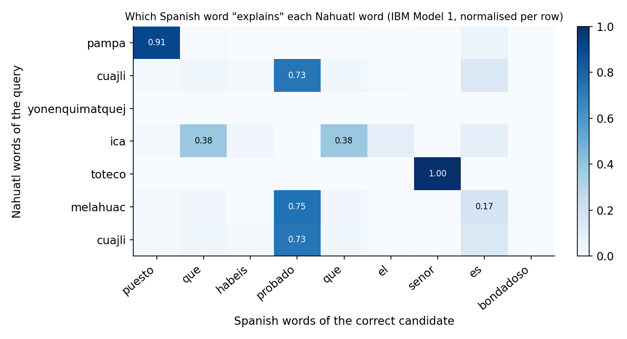
IBM Model 1 alignment between a validation query and its correct translation

The figure shows the learned table on a validation pair ("since you have tasted that the Lord is good"). Some alignments are spot on: pampa with puesto (from "puesto que", "since"), toTeco ("our Lord") with Señor. Others are approximate: cuajli ("good") sits on probado instead of bondadoso. The long verb yonenquimatquej was never seen in training, so it contributes the same small penalty to every candidate and does not affect the ranking. Even this imperfect alignment is enough: the correct translation explains the query far better than the 9 others.

Which direction? You can also train the reverse model $P(E \mid F)$ , where Nahuatl words generate Spanish ones. It is clearly worse (79.6 % on test against 90.8 %). A likely reason is the agglutination: a Nahuatl verb with 4 morphemes corresponds to 3 or 4 Spanish words, and Model 1 lets each generated word pick its own source. When Nahuatl is generated from Spanish, one long Nahuatl word only needs one good Spanish source. When Spanish is generated from Nahuatl, every Spanish article, preposition and pronoun has to be explained by something, and the many rare Nahuatl word forms are poor, sparse sources.

The full solution

Tokenise: lowercase, remove accents (Jesús and Jesus become one token), split on non-letters. Nothing else, no stemming.
Train IBM Model 1 for $P(\text{nahuatl} \mid \text{spanish})$ with 8 EM iterations on the 10 000 training pairs (about 40 seconds of pure Python with dictionaries).

for f in F:                                   # each Nahuatl word of a pair
    w = [t[f].get(e, 1e-9) for e in E]        # E = Spanish words + NULL
    z = sum(w)
    for e, we in zip(E, w):
        count[f][e] += we / z                 # E-step: soft alignment
        total[e] += we / z
# M-step: t[f][e] = count[f][e] / total[e]

Score the 10 candidates of each query with four signals: the Model 1 log-probability in both directions, the shared-word score and the length prior.
Mix them linearly, $s = s_{\text{IBM}} + w_1 s_{\text{shared}} + w_2 s_{\text{length}} + w_3 s_{\text{reverse}}$ , with the three weights chosen by a small grid search on the validation set. The best weights are $w_1 = 0.1$ , $w_2 = 0.3$ , and $w_3 = 0$ : the reverse model adds nothing once the forward one is there. Three weights tuned on 500 queries cannot overfit much, and validation and test agree within 2 points.
Answer with the arg max.

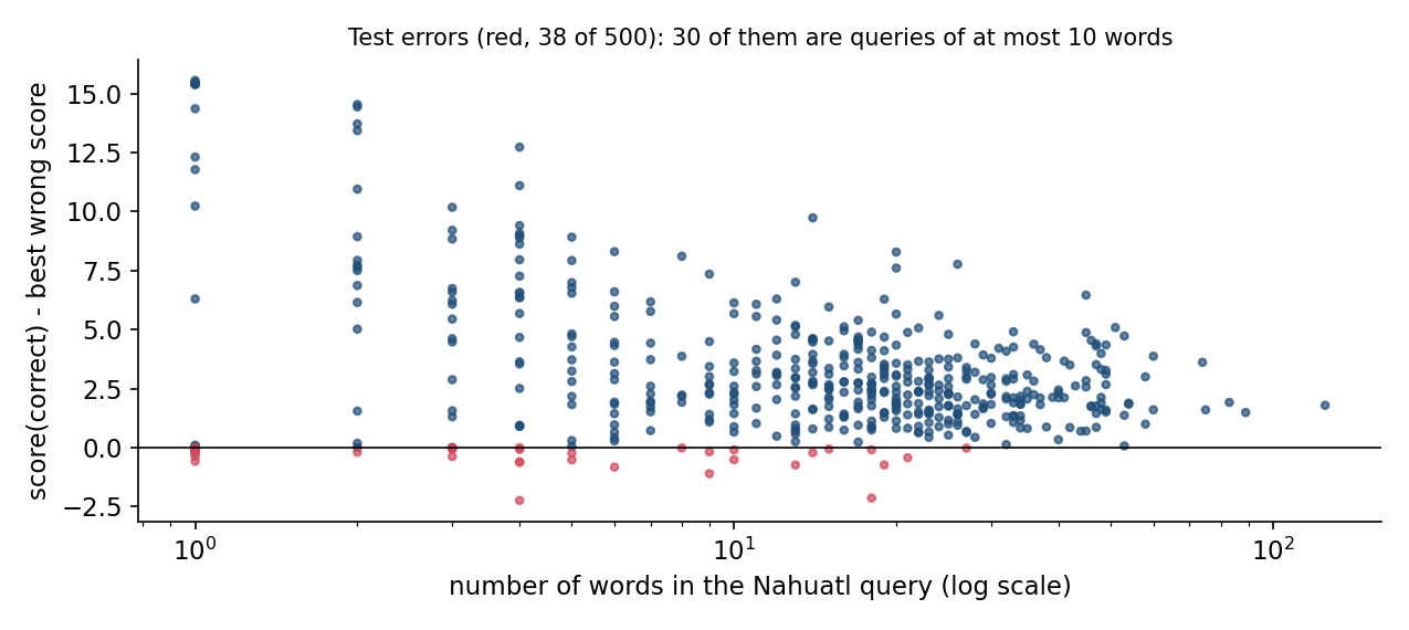
Margin of the correct candidate on the test set, against query length

Where does it still fail? The plot shows, for each test query, the score of the correct candidate minus the best wrong score: positive means success. Errors concentrate on short queries. Of the 172 queries with at most 10 words, 30 are wrong (17 %); of the 328 longer ones, only 8 (2.4 %). One-word queries (often dictionary entries, such as a plant name) fail 12 times out of 33. That makes sense: a long sentence gives Model 1 dozens of independent pieces of evidence, while one unseen word gives it nothing, and the only signals left are length and copied letters.

Results

approach	validation	test
random choice	10 %	10 %
length prior only	19.4 %	21.2 %
organisers' baseline: MiniLM multilingual embeddings, cosine	33.6 %	34.6 %
shared words (names, numbers, loanwords)	53.0 %	54.6 %
IBM Model 1, $P(\text{spanish} \mid \text{nahuatl})$	79.6 %	79.6 %
IBM Model 1, $P(\text{nahuatl} \mid \text{spanish})$	93.0 %	90.8 %
final: IBM-1 + shared words + length prior	94.6 %	92.4 %
final + "known distractor" filter (dataset artefact, see below)	95.4 %	94.6 %

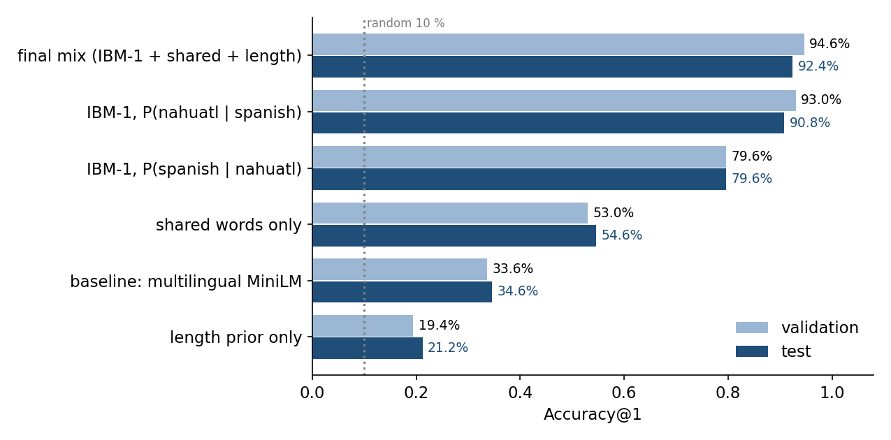
Accuracy of each approach on validation and test

Two things we tried and stopped. Comparing more pretrained encoders (LaBSE, multilingual E5) and fine-tuning MiniLM on the training pairs with a contrastive loss were both started, then cancelled because the shared machine was overloaded. They are the natural "deep learning" route: fine-tuning a sentence encoder with in-batch negatives on 10 000 pairs is standard. But a 1993 statistical model trained in 40 seconds on a CPU already gets 92 %, and any neural model would have to learn the same word correspondences from the same 10 000 pairs.

The dataset artefact. The distractors were sampled from translations of other sentences, and many of those sentences are in the training set. So if a candidate appears in training_set.csv paired with a different Nahuatl sentence, it is almost surely a distractor. Removing such candidates lifts the test score to 94.6 %. We do not use this in the final model: it exploits how the organisers built the task, not anything about Nahuatl, and it would vanish on genuinely new data. It is still worth spotting. In a competition, checking how negatives were generated is part of understanding the data, and organisers should deduplicate distractors against the training set.

What to remember

Ask what the pretrained model has actually seen. A multilingual encoder that never saw Nahuatl reaches 34 %. When the language (or domain) is out of distribution, the labelled data you were given is the real resource.
Parallel sentences are a hidden dictionary. IBM Model 1 with EM recovers word translations (agua → atl) from co-occurrence alone, with no initial dictionary. It is a clean example of EM on hidden variables: here, which word produced which.
Choose the direction of a generative score carefully. Ranking candidates by $P(\text{query} \mid \text{candidate})$ compares every candidate on the same thing to explain. And the direction where each long agglutinated word only needs one source fits the model best.
Cheap signals stack. Copied names and numbers, and a length prior, add 1.6 points on top of the translation model. Measure each signal alone first, then combine with a few weights tuned on validation.
Look at how negatives were made. Distractors reused from the training set create a shortcut. Spot it, report it, and keep it out of a model meant to generalise.

"""
Bulgaria NCAI 2026 final, Task 2: Nahuatl -> Spanish sentence retrieval (pick 1 of 10 candidates).

Data (personal mirror of the official files): github.com/yonitoo/awesome-BGOAI-tasks, 2026/NCAI/R2/Task_2
  training_set.csv (10 000 pairs), validation_set.csv + ground_truth_validation.csv,
  test_set.csv + ground_truth_test.csv. Put them in DATA_DIR.

Idea: learn a word translation table from the 10 000 parallel pairs with IBM Model 1 (EM), then score each
candidate by how well it "explains" the Nahuatl sentence, P(nahuatl | spanish). Two cheap extra signals
(shared words such as names, numbers, loanwords; and a length prior) are mixed in with 2 weights chosen on
the validation set. The test set is scored once, at the end. No neural network, CPU only, ~5 minutes.
"""
import os, re, math, unicodedata, collections, itertools
import numpy as np, pandas as pd

DATA_DIR = os.environ.get("DATA_DIR", "work")
rd = lambda f: pd.read_csv(f"{DATA_DIR}/{f}").fillna("")
train, val, test = rd("training_set.csv"), rd("validation_set.csv"), rd("test_set.csv")
g_val = rd("ground_truth_validation.csv").correct_position.values
g_test = rd("ground_truth_test.csv").correct_position.values
cands = lambda df: [[r[f"spanish_{j}"] for j in range(10)] for _, r in df.iterrows()]
C_val, C_test = cands(val), cands(test)


# ------------------------------------------------------------------ tokenisation
def norm(s):
    """lowercase + strip accents: 'Jesús' and 'Jesus' become the same token"""
    s = unicodedata.normalize("NFKD", s.lower())
    return "".join(c for c in s if not unicodedata.combining(c))

def words(s):
    return re.findall(r"\w+", norm(s))


# ------------------------------------------------------------------ IBM Model 1
def train_model1(src, tgt, iters=8):
    """EM for t[f][e] = P(target word f | source word e). Each source sentence gets a NULL word."""
    t = None
    for _ in range(iters):
        count = collections.defaultdict(lambda: collections.defaultdict(float))
        total = collections.defaultdict(float)
        for E, F in zip(src, tgt):
            E = E + ["<NULL>"]
            for f in F:
                # E-step: each target word is "explained" by the source words in proportion to t(f|e)
                tf = t.get(f, {}) if t is not None else None
                w = [1.0 if t is None else tf.get(e, 1e-9) for e in E]
                z = sum(w)
                for e, we in zip(E, w):
                    count[f][e] += we / z
                    total[e] += we / z
        # M-step: renormalise the soft counts per source word
        t = {f: {e: c / total[e] for e, c in d.items()} for f, d in count.items()}
    return t

def model1_logprob(t, E, F):
    """mean over target words of log P(f | sentence E) = log( 1/(|E|+1) sum_e t(f|e) )"""
    E = E + ["<NULL>"]
    s = 0.0
    for f in F:
        tf = t.get(f)
        p = sum(tf.get(e, 0.0) for e in E) / len(E) if tf else 0.0
        s += math.log(p + 1e-7)          # unseen Nahuatl word: same small penalty for every candidate
    return s / max(1, len(F))

sp_tr = [words(s) for s in train.spanish]
na_tr = [words(s) for s in train.nahuatl]
print("training IBM Model 1, both directions ...")
t_n_given_s = train_model1(sp_tr, na_tr)   # P(nahuatl word | spanish word)
t_s_given_n = train_model1(na_tr, sp_tr)   # P(spanish word | nahuatl word)


# ------------------------------------------------------------------ candidate scores
log_ratio = np.log((train.spanish.str.len() + 5) / (train.nahuatl.str.len() + 5))
mu, sd = log_ratio.mean(), log_ratio.std()

def feats(df, C):
    """returns 4 score matrices (queries x 10 candidates)"""
    out = np.zeros((4, len(df), 10))
    for i, (q, cs) in enumerate(zip(df.nahuatl, C)):
        F = words(q); Fset = {w for w in F if len(w) >= 3}
        for j, c in enumerate(cs):
            E = words(c)
            out[0, i, j] = model1_logprob(t_n_given_s, E, F)                 # does c explain q ?
            out[1, i, j] = model1_logprob(t_s_given_n, F, E)                 # does q explain c ?
            out[2, i, j] = len(Fset & {w for w in E if len(w) >= 3}) / math.sqrt(1 + len(set(E)))  # copied words
            z = (math.log((len(c) + 5) / (len(q) + 5)) - mu) / sd
            out[3, i, j] = -0.5 * z * z                                       # Gaussian length prior
    return out

Fv, Ft = feats(val, C_val), feats(test, C_test)
acc = lambda S, g: float((S.argmax(1) == g).mean())
names = ["P(nah|sp)", "P(sp|nah)", "shared words", "length prior"]
for k in range(4):
    print(f"{names[k]:14s} alone   val {acc(Fv[k], g_val):.3f}   test {acc(Ft[k], g_test):.3f}")

# ------------------------------------------------------------------ combine (weights chosen on validation)
grid = [0, 0.1, 0.2, 0.3, 0.5, 0.75, 1.0]
best = max(itertools.product(grid, grid, grid),
           key=lambda w: (acc(Fv[0] + w[0] * Fv[1] + w[1] * Fv[2] + w[2] * Fv[3], g_val), -sum(w)))
mix = lambda F: F[0] + best[0] * F[1] + best[1] * F[2] + best[2] * F[3]
print("weights (P(sp|nah), shared, length):", best)
print(f"FINAL  val {acc(mix(Fv), g_val):.3f}   test {acc(mix(Ft), g_test):.3f}")

# Dataset artefact (reported, NOT used in the final model): distractors were drawn from the training
# pairs, so a candidate that appears in train with a different Nahuatl sentence is almost surely wrong.
pair = dict(zip(train.spanish, train.nahuatl))
leak = lambda df, C: np.array([[-100.0 if (c in pair and pair[c] != q) else 0.0 for c in cs]
                               for q, cs in zip(df.nahuatl, C)])
print(f"with the leak  val {acc(mix(Fv) + leak(val, C_val), g_val):.3f}   "
      f"test {acc(mix(Ft) + leak(test, C_test), g_test):.3f}")

pd.DataFrame(mix(Ft).argmax(1)).to_csv("Task_2_submission.csv", index=False, header=False)
np.save(f"{DATA_DIR}/feats_val.npy", Fv); np.save(f"{DATA_DIR}/feats_test.npy", Ft)
for s in ["dios", "agua", "casa", "tierra", "corazon"]:     # a peek at the learned lexicon
    col = sorted(((d.get(s, 0), f) for f, d in t_n_given_s.items()), reverse=True)[:4]
    print(s, "->", ", ".join(f"{f} ({p:.2f})" for p, f in col))

Nahuatl–Spanish Sentence Retrieval