IOAI Training: Learn AI by solving problems

The problem in brief

A factory inspects four kinds of products (the images behind them are bottles, cables, capsules and hazelnuts from the MVTec AD benchmark), but you never see the images: each product photo has already been turned into a $37\times 37$ grid of 768-dimensional patch embeddings. For each category you get an "atlas" of about 2 000 embeddings of normal patches, plus 160 normal calibration images. Products come from two regimes (shift_id 0 or 1) that change the embeddings without meaning a defect. Without any training, you must write four small functions: a $37\times 37$ heatmap of "how anomalous is each patch", a smoothing step, an image-level alarm, and per-category, per-regime thresholds computed from the calibration images. Only torch and numpy are allowed. The final test images are hidden; 23 labelled validation images (16 defective, 7 normal) are public.

The data was downloaded from the organisers' public Drive links in the notebook. The .pt files are pickles from a third party, so we opened them once in a sandbox and converted them to NumPy arrays.

How you are scored

The hidden test set is scored with

S = \tfrac12\Big(\text{AUC}_\text{img} + \text{AUC}_\text{pix} + 0.2\,(\text{F1}_\text{img} + \text{F1}_\text{pix})\Big),

so the maximum is $1.2$ . $\text{AUC}_\text{img}$ ranks images by their alarm, and $\text{AUC}_\text{pix}$ ranks all patches of all images pooled together by their heatmap value, against the defect masks. The evaluation code divides every alarm by tau_img and every heatmap by tau_pix of the image's (category, regime) before computing anything. The two F1 scores need a hard decision; the statement does not spell out the rule, and we read it as "defective when score / tau > 1", which is what the division by tau suggests. Only the AUCs can be checked on the public validation set according to the statement; we also compute the F1s with that rule.

No baseline, threshold or leaderboard is published, so there is no official target. For reference: the template functions (heatmap of zeros) score $0.5$ , and a perfect answer scores $1.2$ .

First look at the data

Two scales are mixed in the data, and both break a naive method.

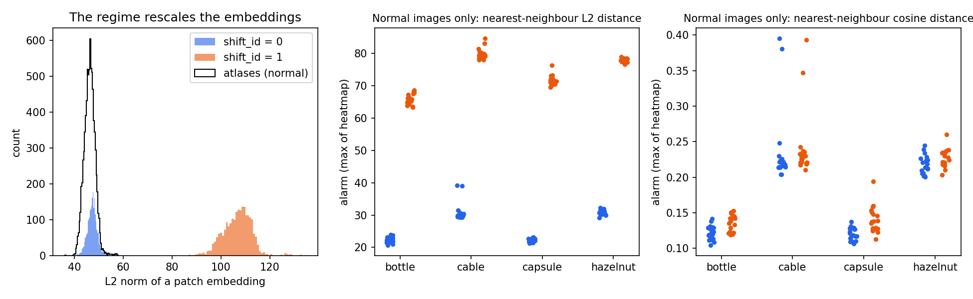
The regime rescales embeddings; L2 alarms depend on regime and category, cosine alarms only on category

The regime multiplies the embeddings by about 2.3. In regime 0, patches have an L2 norm near 47, like the atlas. In regime 1 the norm is near 105 and the per-dimension spread is 2.3 times larger, while the direction of the mean embedding barely moves (cosine 0.86 to 0.94 with the atlas mean in both regimes). So regime 1 is essentially "the same picture, louder", with a little extra noise.
Categories differ in how far normal patches sit from their atlas. Even for perfectly normal images, the nearest-neighbour distance is about twice as large for cables and hazelnuts as for bottles and capsules (right panel), simply because their textures vary more and 2 000 atlas patches cover them less densely.

The middle panel shows the consequence for a plain L2 nearest-neighbour detector: every normal image of regime 1 has a higher alarm (65 to 85) than any normal image of regime 0 (20 to 40). Since $\text{AUC}_\text{img}$ ranks all images together, a normal regime-1 cable outranks a defective regime-0 bottle.

A first baseline

The classic training-free detector (the idea behind PatchCore) scores each patch by its distance to the nearest normal patch in the atlas:

h(x) = \min_{a \in \text{atlas}} \lVert x - a \rVert_2, \qquad \text{alarm} = \max_{\text{patches}} h.

On the 23 validation images, with raw scores, this gives $\text{AUC}_\text{img} = 0.683$ and $\text{AUC}_\text{pix} = 0.754$ . Without thresholds every F1 is 0, so $S \approx 0.72$ . The detector itself works (inside one category and one regime, defects do stand out), but its scores live on eight different scales.

The key idea

Make the score invariant to what you know is not a defect, then express it in units of "how high a normal example can go".

Step 1: remove the regime with the cosine distance. If regime 1 is roughly $x \mapsto 2.3\,x$ , then any score that depends on the length of the vectors moves with it, while a score that depends only on their direction does not. The cosine distance to the nearest atlas patch,

h(x) = 1 - \max_{a \in \text{atlas}} \frac{x \cdot a}{\lVert x\rVert\,\lVert a\rVert},

is unchanged when $x$ is multiplied by any positive number. The right panel of the figure shows that the two regimes now overlap almost perfectly inside each category. On validation this alone raises the raw $\text{AUC}_\text{img}$ from 0.683 to 0.881 and the raw $\text{AUC}_\text{pix}$ from 0.754 to 0.978.

Step 2: put the categories on one scale with calibration. The remaining difference between categories is real (cable patches are harder to match), but a defect means "far from normal for this category". The calibration set gives, for every (category, regime) pair, 20 normal images. We set

\tau_\text{img} = \max_{\text{normal calib. images}} \text{alarm}, \qquad \tau_\text{pix} = \max_{\text{normal calib. patches}} h.

After division, a value of 1 means "as high as the most suspicious normal example we have ever seen". This does two things at once. It aligns the scales, which is what pooled AUCs need, and it gives a natural hard decision for the F1 scores (score / tau $> 1$ ) without peeking at a single defective example. Using the maximum rather than a quantile keeps the false-alarm rate on normal products low, which is the cautious choice when the test distribution is unknown.

Why not tune the thresholds on the validation images? Because there are only 16 defective ones, the statement explicitly warns that the hidden test is different, and the calibration rule above has no free parameter fitted on defects.

The full solution

Heatmap: normalise patch and atlas embeddings to unit length, take the largest cosine similarity of each patch to the atlas (one $1369 \times 2000$ matrix product), and return $1 -$ that value as a $37\times 37$ map.

Xn, An = F.normalize(X, dim=1), F.normalize(atlas, dim=1)
heat = (1 - (Xn @ An.T).max(dim=1).values).view(37, 37)

Smoothing: a separable Gaussian blur with $\sigma = 1$ patch (replicate padding). Defects cover connected regions, so averaging with the neighbours removes isolated noisy patches. It raises $\text{AUC}_\text{pix}$ (0.985 to 0.994 on validation) but costs some pixel F1; $\sigma = 2$ is clearly too much (it blurs 3-patch capsule cracks away).
Alarm: the maximum of the smoothed map. A defect is local, so the single worst region decides; the mean of the top 10 patches behaved the same.
Calibration: for each (category, regime), run steps 1 to 3 on the 20 normal images and keep the largest alarm and the largest patch value.

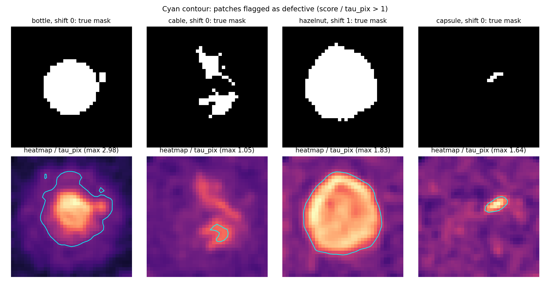
Ground-truth masks and calibrated heatmaps on four validation images

The heatmaps follow the masks closely for large defects (the contaminated bottle, the cracked hazelnut in regime 1). The cable with a bent wire is the hard case: its normalised maximum is only 1.05, so it is barely flagged, and only part of the region crosses the threshold. That case is where most of the pixel-F1 loss comes from.

Results

"Val" is the 23 public validation images. Because 7 normal images are too few to measure false alarms, we also ran a 2-fold check: calibrate on 10 of the 20 normal images of each group, add the other 80 normal calibration images (empty masks) to the validation set, swap, and average. The hidden test labels are private, so these are estimates.

approach	AUC img	AUC pix	F1 img	F1 pix	$S$
template (zeros)	0.5	0.5	0	0	0.50
L2 nearest neighbour, raw scores (val)	0.683	0.754	0	0	0.72
cosine nearest neighbour, raw scores (val)	0.881	0.978	0	0	0.93
L2 + per-group tau (val)	0.960	0.987	0.923	0.680	1.134
L2 after rescaling each image to the atlas norm, + tau (val)	0.992	0.997	0.963	0.683	1.159
cosine, 3 nearest neighbours, + tau (val)	0.992	0.992	0.880	0.792	1.160
cosine, no smoothing, + tau (val)	1.000	0.985	0.963	0.763	1.165
cosine + $\sigma=1$ smoothing + max-calibrated tau (final, val)	1.000	0.994	1.000	0.764	1.174
final, val + 80 held-out normals (2-fold)	0.992	0.998	0.803	0.687	1.144

On the public validation images the final method separates every defective image from every normal one and reaches $S = 1.174$ out of 1.2. The larger 2-fold check is the more honest estimate for a hidden test: $S \approx 1.14$ . The AUCs stay near 0.99, and the drop comes from the F1 scores: with only 10 calibration images per group, a few held-out normal images exceed the calibrated maximum and raise false alarms. On the hidden test, with all 20 calibration images per group, the thresholds should be slightly safer.

What to remember

Find out what the nuisance does to the data, then pick an invariant score. Here the regime was a rescaling, so a scale-free distance (cosine) removed most of it. Look at norms, means and spreads per group before choosing a distance.
Pooled metrics need comparable scores. An AUC computed over several categories and regimes punishes any per-group offset, even if the detector is perfect inside each group.
Calibrate on normals only, with a rule that has no free parameter tuned on defects. "Divide by the highest score a normal example reached" aligns scales and gives a hard threshold in one move.
Nearest-neighbour distance to a bank of normal features is a strong training-free anomaly detector, and smoothing the patch map exploits the fact that real defects are connected regions.
With 23 validation images, differences of 0.01 are noise. Enlarge the evaluation with whatever labelled data you have (here, held-out normal images) before trusting a ranking of variants.

"""Training-free defect localisation in latent space (Bulgaria NCAI 2026, final round, task 3).

The four notebook functions (torch only, no disk access, no training):
  compute_heatmap   : cosine distance of each patch embedding to its nearest neighbour in the
                      normal atlas (cosine ignores the x2.3 scaling that shift_id=1 applies)
  smooth_heatmap    : separable Gaussian blur, sigma = 1 patch
  compute_alarm     : max of the smoothed heatmap
  calibrate_thresholds : per (atlas_id, shift_id), tau = highest score reached by any NORMAL
                      calibration image (image level) or patch (pixel level); dividing by tau puts
                      all categories and regimes on one common scale, and score/tau > 1 = defect.

Data (gdown ids from the notebook): val_data.zip 1z-aeaEwY9yp47x2UFrCzrKD7leVM5OrW, data.zip
1HyyI-0oB72E8ak1X3gQZrMgdExGlQ7oB. The .pt files come from a third party: convert them once inside
the sandbox (run_sandboxed.sh . python3 solution.py --convert) to npy/, then run normally.
Evaluation: AUCs as in the notebook on the 23 public val images; F1 with the threshold score/tau > 1
(our reading of the rules: the hidden test is private); plus a 2-fold check that adds 80 held-out
normal calibration images.
"""
import json, os, sys
import numpy as np, torch, torch.nn.functional as F

# ---------------------------------------------------------------- the four required functions
@torch.no_grad()
def compute_heatmap(X: torch.Tensor, atlas: torch.Tensor) -> torch.Tensor:
    Xn = F.normalize(X.float(), dim=1)               # direction only: robust to the regime's scaling
    An = F.normalize(atlas.float(), dim=1)
    nearest = (Xn @ An.T).max(dim=1).values          # cosine similarity to the closest normal patch
    return (1 - nearest).view(37, 37)                # anomaly = far from every normal patch

@torch.no_grad()
def smooth_heatmap(heatmap: torch.Tensor, sigma: float = 1.0) -> torch.Tensor:
    r = int(3 * sigma + 0.5)
    x = torch.arange(-r, r + 1, dtype=torch.float32)
    g = torch.exp(-x ** 2 / (2 * sigma ** 2)); g = g / g.sum()
    h = F.pad(heatmap[None, None].float(), (r, r, r, r), mode="replicate")
    h = F.conv2d(h, g.view(1, 1, 1, -1)); h = F.conv2d(h, g.view(1, 1, -1, 1))
    return h[0, 0]

@torch.no_grad()
def compute_alarm(heatmap: torch.Tensor) -> float:
    return float(heatmap.max().item())

@torch.no_grad()
def calibrate_thresholds(calibration_data):
    img, pix = {}, {}
    for item in calibration_data:
        key = (int(item["atlas_id"]), int(item["shift_id"]))
        heat = smooth_heatmap(compute_heatmap(item["X"], item["atlas"]))
        img.setdefault(key, []).append(compute_alarm(heat))
        pix.setdefault(key, []).append(float(heat.max()))
    thresholds = {}
    for (a, s) in img:
        # highest score ever reached by a normal example of this category and regime
        thresholds.setdefault(a, {})[s] = {"tau_img": max(img[(a, s)]), "tau_pix": max(pix[(a, s)])}
    return thresholds

# ---------------------------------------------------------------- data handling and evaluation
def convert():
    """Run ONLY inside the sandbox: .pt (pickle) -> .npy."""
    os.makedirs("npy", exist_ok=True)
    for k in range(4):
        np.save(f"npy/atlas_{k}.npy", torch.load(f"data/atlas_{k}.pt", map_location="cpu").float().numpy())
    cal = torch.load("data/calibration.pt", map_location="cpu")
    np.save("npy/calib_X.npy", np.stack([c["X"].float().numpy() for c in cal]).astype(np.float16))
    np.save("npy/calib_meta.npy", np.array([[int(c["atlas_id"]), int(c["shift_id"])] for c in cal]))
    X, M, meta = [], [], []
    for e in json.load(open("val_data/val_manifest.json")):
        d = torch.load(e["file"], map_location="cpu")
        X.append(d["X"].float().numpy()); M.append(d["mask"].numpy().astype(np.uint8))
        meta.append([int(e["atlas_id"]), int(e.get("shift_id", 0)), int(bool(d.get("is_anomaly", False)))])
    np.save("npy/val_X.npy", np.stack(X).astype(np.float16)); np.save("npy/val_mask.npy", np.stack(M))
    np.save("npy/val_meta.npy", np.array(meta))

def auc(y, s):
    from sklearn.metrics import roc_auc_score
    return float(roc_auc_score(y, s))

def f1(y, pred):
    y, pred = np.asarray(y, bool), np.asarray(pred, bool)
    tp = (y & pred).sum(); return float(2 * tp / max(y.sum() + pred.sum(), 1))

def evaluate(items, thresholds, use_tau=True):
    """items: (X, atlas, atlas_id, shift_id, is_anomaly, mask). Returns the 4 metrics + final score."""
    yi, si, yp, sp = [], [], [], []
    for X, atlas, a, s, y, mask in items:
        heat = smooth_heatmap(compute_heatmap(X, atlas))
        t = thresholds[a][s] if use_tau else {"tau_img": 1.0, "tau_pix": 1.0}
        yi.append(y); si.append(compute_alarm(heat) / t["tau_img"])
        yp.append(mask.reshape(-1)); sp.append(heat.reshape(-1).numpy() / t["tau_pix"])
    yp, sp, si = np.concatenate(yp), np.concatenate(sp), np.array(si)
    ai, ap, fi, fp = auc(yi, si), auc(yp, sp), f1(yi, si > 1), f1(yp, sp > 1)
    return ai, ap, fi, fp, 0.5 * (ai + ap + 0.2 * (fi + fp))

if __name__ == "__main__":
    if "--convert" in sys.argv: convert(); sys.exit()
    torch.set_num_threads(2)
    atlases = {k: torch.tensor(np.load(f"npy/atlas_{k}.npy")).float() for k in range(4)}
    CX, CM = np.load("npy/calib_X.npy"), np.load("npy/calib_meta.npy")
    calib = [{"X": torch.tensor(CX[i]).float(), "atlas": atlases[CM[i, 0]], "atlas_id": int(CM[i, 0]),
              "shift_id": int(CM[i, 1])} for i in range(len(CM))]
    VX, VM, VMeta = np.load("npy/val_X.npy"), np.load("npy/val_mask.npy"), np.load("npy/val_meta.npy")
    val = [(torch.tensor(VX[i]).float(), atlases[VMeta[i, 0]], int(VMeta[i, 0]), int(VMeta[i, 1]),
            int(VMeta[i, 2]), VM[i]) for i in range(len(VX))]

    th = calibrate_thresholds(calib)
    for name, use in [("raw scores (no tau)", False), ("scores / tau", True)]:
        r = evaluate(val, th, use)
        print(f"val, {name:20s}: AUCimg {r[0]:.3f} AUCpix {r[1]:.3f} F1img {r[2]:.3f} F1pix {r[3]:.3f} final {r[4]:.4f}")

    # 2-fold check: calibrate on half of the normal images of each group, add the other half
    # (80 normal images with empty masks) to the 23 val images, then swap the halves.
    rank, seen = [], {}
    for a, s in CM: seen[(a, s)] = seen.get((a, s), -1) + 1; rank.append(seen[(a, s)])
    res = []
    for fold in (0, 1):
        cal = [c for c, r in zip(calib, rank) if r % 2 == fold]
        extra = [(c["X"], c["atlas"], c["atlas_id"], c["shift_id"], 0, np.zeros((37, 37), np.uint8))
                 for c, r in zip(calib, rank) if r % 2 != fold]
        res.append(evaluate(val + extra, calibrate_thresholds(cal)))
    r = np.mean(res, 0)
    print(f"val + 80 held-out normals (2-fold): AUCimg {r[0]:.3f} AUCpix {r[1]:.3f} F1img {r[2]:.3f} F1pix {r[3]:.3f} final {r[4]:.4f}")

Training-Free Statistical Defect Localisation in Latent Space