IOAI Training: Learn AI by solving problems

The problem in brief

You get 800 students described by 38 columns (study hours, sleep, IQ, attendance, family income, favourite subject, number of pets...) together with their final test score, and you must predict the score of 800 other students. The statement walks you through the classical toolbox: impute missing values, scale the features, try Ridge and Lasso. The real lesson is elsewhere. Look at the data closely enough and you find that the target is a simple formula, and that the "new" students are not new at all.

The data are the official Kaggle files. The test labels are private and we did not submit anything. Our scores come from cross-validation on the training set, and from a self-made copy of the test that mimics its construction exactly.

How you are scored

The coefficient of determination on the test scores $y_i$ :

R^2 = 1 - \frac{\sum_i (y_i - \hat y_i)^2}{\sum_i (y_i - \bar y)^2}.

$R^2 = 1$ is a perfect prediction; predicting the mean everywhere gives 0.

What to aim for. No threshold is published. On the public leaderboard three entries have $R^2 = 1.000$ , followed by 0.997.

First look at the data

There are no missing values in either file, despite the statement's long section on imputation.
The training columns look like real survey answers: integers for attendance, binary 0/1 for part-time job, gender, favourite subject. The test columns do not: attendance 85.498, homework completed 0.106, gender $-0.19$ , a negative number of pets. Every test value looks like a clean value plus a little random noise.
The scores lie between 55 and 100, with 5 students at exactly 100 (a cap).

A first baseline

Plain linear regression, 5-fold cross-validation on the training set: $R^2 = 0.9994$ . The fit is almost perfect, and the coefficients explain why:

Coefficients and the twin test

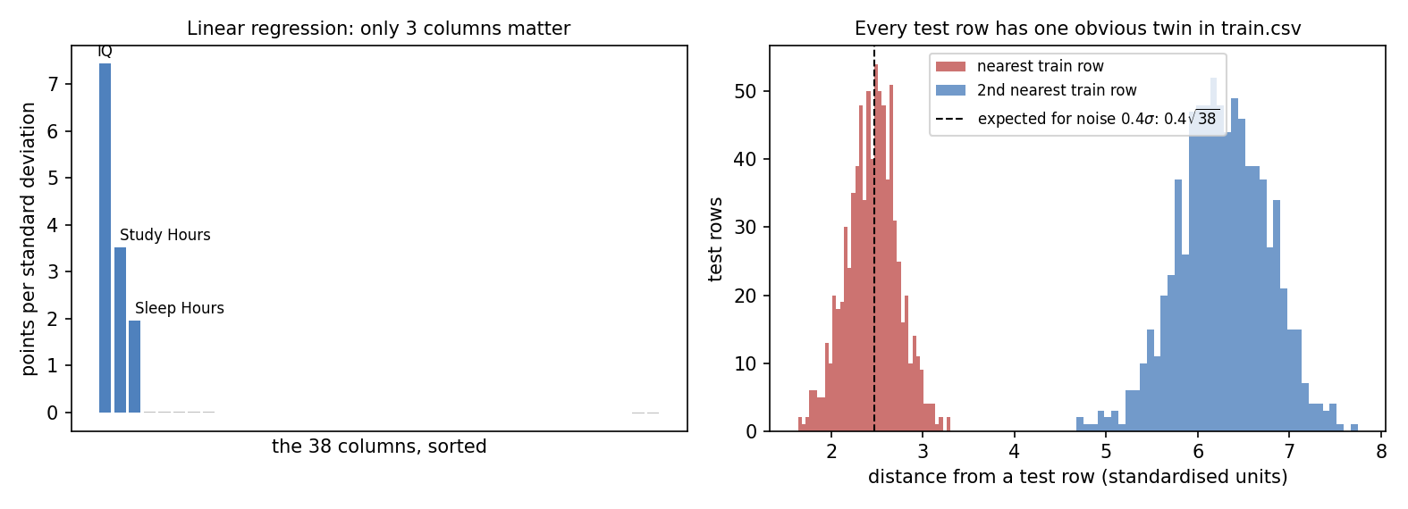
Only IQ (7.4 points per standard deviation), Study_Hours (3.5) and Sleep_Hours (2.0) matter. The other 35 columns have coefficients near 0.01: they are decoys from the data generator. The remaining 0.05 % of variance is the cap at 100. Lasso, the statement's suggestion for feature selection, does worse here (0.87 with the default cross-validated penalty), because it shrinks the three true coefficients along with the useless ones.

But the test rows are noisy, and a model fitted on clean rows does not see the same inputs at test time. To measure what really happens, we add noise of the same size to the validation rows (see below how we measured it). The linear model then drops to $R^2 = 0.855$ .

The key idea

Ask how a test row relates to the training rows before you model anything. For each test row, compute its distance to every training row after standardising the columns. The right panel above shows the result: every test row has one training row at distance about 2.5, and the next closest is at about 6.3. There is no overlap at all between the two histograms, and the 800 nearest neighbours are 800 different training rows.

That is exactly what you would see if the test set were the training set, shuffled, with independent Gaussian noise added to every column. Check the numbers: if each of the 38 standardised columns gets noise of standard deviation $\sigma_u$ , the distance to the original row is about $\sigma_u \sqrt{38}$ . The measured spread of (test minus matched train) is $\sigma_u = 0.40$ in every single column, and $0.40 \sqrt{38} = 2.47$ , which is exactly where the red histogram peaks. Two unrelated students, on the other hand, differ by about $\sqrt{2 \cdot 38} \approx 8.7$ before noise, and the closest of 800 of them is around 6.

So the test students are the training students in disguise. Matching each test row to its twin and copying the twin's score gives the exact answer. To make the matching one-to-one, we solve an assignment problem: find the permutation $\pi$ that minimises

\sum_{i} \lVert z_i - x_{\pi(i)} \rVert^2,

where $z_i$ are the standardised test rows and $x_j$ the training rows, with the Hungarian algorithm (scipy.optimize.linear_sum_assignment). Here it agrees with the plain nearest neighbour on all 800 rows, because the gap between first and second neighbour is so large.

Why can no model reach $R^2 = 1$ on these test rows? It is the errors-in-variables effect. Suppose, in standard units, $y = \beta x$ and you observe $z = x + u$ with noise variance $\lambda^2 = 0.16$ . The best you can do from $z$ is

\mathbb{E}[y \mid z] = \frac{\beta}{1 + \lambda^2}\, z,

which explains only a fraction

R^2_{\max} = \frac{1}{1 + \lambda^2} = \frac{1}{1.16} \approx 0.862

of the variance. This holds feature by feature, so it holds for the whole linear score too. Training on noisy copies of the training rows learns exactly this shrunken slope, and reaches 0.872 in our cross-validation (the small excess over 0.862 is sampling noise). The information lost to the noise in IQ is gone. It can only be recovered by finding the clean row the noise was added to.

The full solution

Standardise the 38 columns with the training means and standard deviations.
Compute all $800 \times 800$ squared distances between test and training rows.
Solve the assignment problem, and predict for each test row the Test_Score of its assigned training row.

How we validated the matching. We built a self-made test: the training set shuffled, plus Gaussian noise of 0.4 standard deviations in every column. The assignment recovered 100 % of the rows, so $R^2 = 1.000$ . It still recovers 100 % with noise of 1.0 standard deviation, and breaks down at 2.0 (37 % of rows): the method has a wide safety margin. On the real test, a last consistency check: the scores we copy and the linear model's predictions on the noisy test rows agree with $R^2 = 0.852$ , the same value as our noisy cross-validation (0.855), as expected if the copied scores are the truth.

Results

approach	$R^2$	evaluated on
Lasso, cross-validated penalty, clean validation	0.868	5-fold CV
linear regression, all columns, clean validation	0.9994	5-fold CV
gradient boosting, clean validation	0.984	5-fold CV
linear regression, all columns, noisy validation	0.855	5-fold CV + test-like noise
gradient boosting, noisy validation	0.838	5-fold CV + test-like noise
linear, 3 key columns, trained on noisy copies	0.872	5-fold CV + test-like noise
theoretical ceiling for any model of the noisy inputs	0.862	formula above
twin matching (assignment), final	1.000	self-made noisy shuffled copy

The public leaderboard's top score of 1.000 is consistent with this: the leading teams evidently found the same thing.

Is this fair play? The statement does not forbid it, and the test data reveal it to anyone who looks. As a lesson about real projects, it is a classic train/test leakage story: if your "new" data are noisy duplicates of your training data, any score you measure on them says nothing about new students. Always check for near-duplicates between your splits.

What to remember

Look at the raw test values, not just the training ones. Integers that became decimals, binary columns with negative values: these are signs that the test set was built differently.
Nearest-neighbour distances are a powerful diagnostic. A clear gap between the first and second neighbour means duplicates, and here it turned a regression problem into a matching problem.
Noisy inputs put a ceiling on $R^2$ . With noise variance $\lambda^2$ relative to the signal, the best possible $R^2$ is about $1/(1+\lambda^2)$ . Training on inputs noised the same way learns the right, shrunken coefficients.
Matching with a one-to-one constraint is an assignment problem, solved exactly by the Hungarian algorithm in a fraction of a second for 800 rows.
The statement's checklist is not always the problem's key. There were no missing values, scaling does not change a linear regression, and Lasso hurt. Your own exploration decides what matters.

"""BdAIO 2024, "Ace the Grades": worked solution.

Two findings:
1. The score is (almost exactly) linear in three columns: IQ, Study_Hours and Sleep_Hours
   (training R^2 = 0.9995, the rest is clipping at 100). The other 35 columns are decoys.
2. test.csv is NOT new students: it is train.csv shuffled, with Gaussian noise of 0.4 standard
   deviations added to every column. Each test row has one train row at distance ~2.5 (in standard
   units) and the next one at ~6.3, so a one-to-one assignment (Hungarian algorithm) recovers the
   original row, and its Test_Score, exactly.

The honest model (linear regression, noise-aware) is evaluated by 5-fold CV with the same noise added
to the validation rows; the matching is evaluated on a self-made noisy shuffled copy of train.csv.
Official test labels are private.

Usage: python solution.py [folder with train.csv and test.csv]
"""
import sys
import numpy as np
import pandas as pd
from scipy.optimize import linear_sum_assignment
from scipy.spatial.distance import cdist
from sklearn.linear_model import LinearRegression
from sklearn.metrics import r2_score
from sklearn.model_selection import KFold

D = sys.argv[1] if len(sys.argv) > 1 else "work/bdaio-2024-ace-the-grades"
tr, te = pd.read_csv(f"{D}/train.csv"), pd.read_csv(f"{D}/test.csv")
F = [c for c in tr.columns if c != "Test_Score"]
X, y = tr[F].values, tr.Test_Score.values
s = X.std(0)
rng = np.random.default_rng(0)
NOISE = 0.4                                    # measured: std(test - matched train) / std(train) per column

# ---------------------------------------------------------------- 1. the regression view
def cv_r2(cols, noisy_val, noisy_train=False, reps=5):
    idx = [F.index(c) for c in cols]
    scores = []
    for a, v in KFold(5, shuffle=True, random_state=0).split(X):
        Xa, ya = X[a][:, idx], y[a]
        if noisy_train:                         # train on noisy copies: learns the attenuated slope
            Xa = np.vstack([Xa + rng.normal(0, NOISE * s[idx], Xa.shape) for _ in range(reps)])
            ya = np.tile(ya, reps)
        Xv = X[v][:, idx] + (rng.normal(0, NOISE * s[idx], (len(v), len(idx))) if noisy_val else 0)
        scores.append(r2_score(y[v], LinearRegression().fit(Xa, ya).predict(Xv)))
    return np.mean(scores)

KEY = ["IQ", "Study_Hours", "Sleep_Hours"]
print(f"linear, all columns, clean validation : {cv_r2(F, False):.4f}")
print(f"linear, all columns, noisy validation : {cv_r2(F, True):.4f}")
print(f"linear, 3 key columns, noisy val      : {cv_r2(KEY, True):.4f}")
print(f"  + trained on noisy copies           : {cv_r2(KEY, True, True):.4f}")

# ---------------------------------------------------------------- 2. the matching view
def match(A, B):
    """Optimal one-to-one assignment of rows of A to rows of B (standardised squared distance)."""
    return linear_sum_assignment(cdist(A / s, B / s, "sqeuclidean"))[1]

perm = rng.permutation(len(X))                  # self-made test: shuffled train + the same noise
fake = X[perm] + rng.normal(0, NOISE * s, X.shape)
col = match(fake, X)
print(f"self-made noisy copy: {np.mean(col == perm):.1%} rows matched, R2 {r2_score(y[perm], y[col]):.4f}")

Dt = np.sqrt(cdist(te[F].values / s, X / s, "sqeuclidean"))
d = np.sort(Dt, 1)
print(f"real test: median distance to 1st / 2nd nearest train row: {np.median(d[:, 0]):.2f} / {np.median(d[:, 1]):.2f}")
col = match(te[F].values, X)
pred = y[col]
lin = LinearRegression().fit(X, y)
print(f"R2 between copied scores and the linear model on noisy test rows: {r2_score(pred, lin.predict(te[F].values)):.3f}")
pd.DataFrame({"ID": te.ID, "Predicted": pred}).to_csv("submission.csv", index=False)
print("wrote submission.csv (not submitted)")