IOAI Training: Learn AI by solving problems

The problem in brief

Somewhere in the square $[-1,1]^2$ sits a single source of a central force field: at every point, the force points straight towards or away from the source, and its signed magnitude $f_s(r)$ depends only on the distance $r$ . The function $f_s$ is unknown and changes from sample to sample (it can be attractive, repulsive, or switch sign with distance). You observe the force vectors on a $64\times 64$ grid and must return the source coordinates and $f_s$ at 100 radii $r_i = 0.02, 0.04, \dots, 2.00$ . There are 10 000 labelled training samples, 2 000 labelled validation samples and 3 000 test samples (USA AI Olympiad 2026, Round 2, Day 1, Problem 2, data on Hugging Face). The test labels are private, so we report the official metric on the validation set, which we never used for fitting or tuning.

How you are scored

Per sample, lower is better:

\text{err}_s = 10^3\,\big(|\hat x_s - x_s| + |\hat y_s - y_s|\big) + 3\cdot 10^{-3}\sqrt{\tfrac{1}{100}\textstyle\sum_i \big(\hat f_s(r_i) - f_s(r_i)\big)^2},

averaged over samples. The final mark is relative: $100\,\frac{X_\text{baseline} - X}{X_\text{baseline} - X_\text{best}}$ , where the baseline is the organisers' CNN that regresses all 102 numbers directly, and $X_\text{best}$ is the better of the jury's expert model and the best contestant. None of these reference scores is published, so there is no number to aim for. As a yardstick we use the trivial " $f \equiv 0$ " prediction (with a perfect source), which scores 102.9 on validation.

The weights tell you what matters. One grid cell is $2/63 \approx 0.032$ , so missing the source by one cell costs about 32 points. In the field term, $f$ near the source reaches $10^5$ to $10^6$ , so the RMSE is completely dominated by the smallest radius.

First look at the data

Three observations change the whole problem.

The sources sit exactly on grid nodes: every training and validation source has coordinates $-1 + 2k/63$ , and the field vector at that node is about $10^{-8}$ .
The sensor saturates. Comparing the observed radial component with the true $f$ : up to $|f| \approx 20$ , the observations equal the truth with roughly 5 % multiplicative noise. Beyond that they flatten at about 25 in absolute value (median ratio observed/true 0.42 for $|f|\in[40,100]$ , and 0.08 above 100). The near field is therefore never observed: all you see there is "big, with this sign".
The metric lives where the data is blind. In our final model, 99.7 % of the squared field error comes from $r = 0.02$ , even though the nearest grid point is 0.032 from the source and the first trustworthy measurement is typically at $r \gtrsim 0.15$ .

Near-source behaviour varies a lot: the local log-log slope between $r=0.02$ and $0.04$ ranges from about 2.3 to 3.9 (10th to 90th percentile), and $|f(0.02)|$ from $3\times10^3$ to $1.2\times10^6$ . No simple law fits all samples. Two power laws plus an exponential factor fit individual curves to within about 2 % (median), but not exactly, which suggests a mixture of families.

A first baseline

Source by geometry. Every vector $\mathbf{F}(\mathbf{p})$ is parallel to $\mathbf{p} - \mathbf{s}$ , so the source lies on the line through $\mathbf{p}$ with direction $\mathbf{u} = \mathbf{F}/\|\mathbf{F}\|$ . That gives one linear equation per grid point, $u_x (s_y - p_y) - u_y (s_x - p_x) = 0$ . Solving the 4096 equations by least squares (reweighted to trust nearby points more) gives an L1 error of 0.0009, a thirtieth of a cell. Snapping to the nearest grid node then recovers every source exactly: 10 000 / 10 000 in training and 2 000 / 2 000 in validation. The source term of the metric is 0.
Field by direct reading. Project each vector on the radial direction, $f_\text{obs} = \mathbf{F}\cdot(\mathbf{p}-\mathbf{s})/\|\mathbf{p}-\mathbf{s}\|$ , average per radius bin, and interpolate. This scores 102.9, no better than predicting zero. Where the metric cares, the observations are saturated at 25 against true values of $10^4$ and more.

The key idea

Physics gives the source for free. The remaining difficulty is a pure extrapolation problem: predict a function's value at $r = 0.02$ from its values where $|f| \lesssim 15$ , typically at $r \ge 0.15$ , so across almost a decade in radius. No formula can do that for an unknown family, but 10 000 examples of the family can. We learn the map

\text{trusted part of the radial profile} \;\longmapsto\; \big(f(r_1), \dots, f(r_{100})\big).

Two choices make this work.

Work in $\operatorname{asinh}$ space. $z = \operatorname{asinh} f$ behaves like $\operatorname{sign}(f)\log(2|f|)$ for large values and like $f$ near zero, so values from $10^{-2}$ to $10^6$ with either sign become numbers between about $-15$ and $15$ that a network can regress.
Use an L1 loss, i.e. predict the median. The metric is close to $|\hat f(0.02) - f(0.02)|/10$ , an absolute error on the raw scale. The prediction that minimises an expected absolute error is the conditional median, and since asinh is monotone, the median of $z$ maps to the median of $f$ . With a squared loss in asinh space, the network learns a geometric-mean-like quantity and its raw-scale error was unstable: it rose from 41 to 215 as training went on.

The full solution

Source: weighted least-squares line intersection, snapped to the grid.
Radial profile: average $f_\text{obs}$ over grid points within $\pm 0.01$ of each $r_i$ . Features: $\operatorname{asinh}$ of the trusted bins ( $|f_\text{obs}| \le 15$ ), a mask of trusted bins, the sign of saturated bins, and the number of points per bin (400 features).
Field: 3 MLPs (two hidden layers of 512 units, dropout 0.2, weight decay 0.01, 80 epochs, L1 loss on standardised $\operatorname{asinh} f$ ), averaged in asinh space. At $r = 0.02$ , this is averaged half and half with a gradient-boosting regressor trained with an absolute-error loss.
For the test set, train on train + validation and write the 102 columns in the sample-submission format.

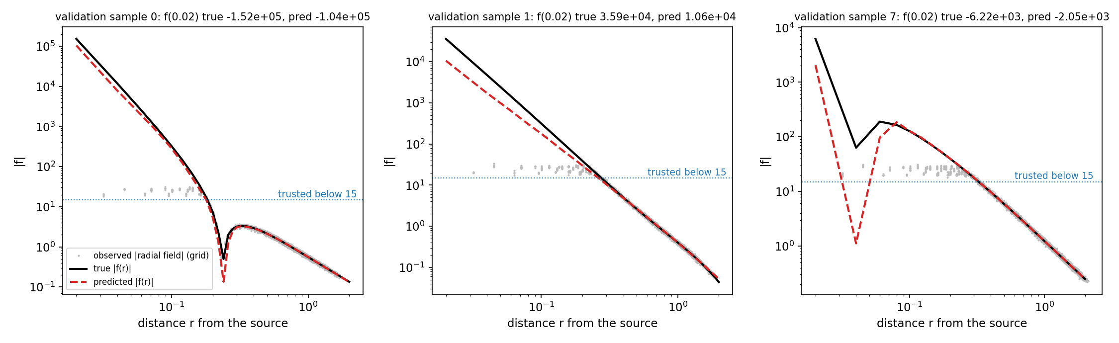
Observed (saturated) profiles, truth and prediction for three validation samples

The grey dots show what the grid really measures: below about $r = 0.2$ to $0.3$ they are stuck between 20 and 30, whatever the truth. Sample 0 is a good case, where the steep rise continues the trend seen in the trusted zone. Sample 1 shows the typical error, a near-field slope that is slightly too shallow. Sample 7 is hopeless: the field changes sign inside the saturated zone, which the data cannot reveal.

Results

Official metric on the 2 000 validation samples. Test labels are private, and the organisers' baseline and expert scores are not published.

approach	source term	field term	score
exact source, $f \equiv 0$	0.00	102.87	102.87
exact source, observed profile read directly	0.00	102.86	102.86
exact source, MLP with MSE loss in asinh space (best epoch / end)	0.00	40.9 / 215.1	40.9 / 215.1
exact source, regularised MLP, MSE loss	0.00	26.8	26.8
exact source, gradient boosting at $r=0.02$ only, MSE / L1 loss	0.00	30.1 / 24.7	30.1 / 24.7
exact source, 3 MLPs with L1 loss	0.00	25.1	25.1
exact source, 3 MLPs + boosting at $r = 0.02$ (final)	0.00	23.75	23.75

The remaining error is uncertainty about how steep $f$ is below the first unsaturated radius. At $r = 0.02$ the ratio of predicted to true value has median 0.93 (interquartile range 0.69 to 1.21). The prediction is within a factor 1.5 of the truth for 67 % of samples and within a factor 2 for 87 %, and the sign is right for 98.3 %.

What to remember

Use the physics first: a central field means every vector points at the source, so the location is a linear least-squares problem, and the grid prior makes it exact.
Look at what the sensor really measures. Saturation turns "fit $f$ " into "extrapolate $f$ ", a completely different problem.
Find where the metric's mass is: here one radius out of 100 carries 99.7 % of the error.
Choose the loss to match the metric. An absolute error calls for the median, which an L1 loss on any monotone transform of the target delivers.
Targets spanning six orders of magnitude and both signs: regress $\operatorname{asinh}(y)$ .

"""USAAIO 2026 Round 2, Problem 2: locate the single source of a central field and recover f(r).

1. Source: every observed vector lies on a line through the source; a weighted least-squares
   intersection of the 4096 lines, snapped to the 64x64 grid (sources sit on grid nodes).
2. Profile: project each vector on the radial direction and average per radius r_i = 0.02 i.
   The sensor saturates near |F| = 25, so only values below 15 are trusted.
3. Extrapolation: the unobservable near field (which dominates the metric) is predicted from
   the trusted profile by 3 MLPs (L1 loss on asinh f, i.e. the conditional median) and, at
   r = 0.02, averaged with a gradient-boosting model (absolute-error loss).
  python3 solution.py --validate     # train on train.npz, score on val.npz
  python3 solution.py                # train on train+val, write submission.csv for the test set
Run from the folder holding train.npz, val.npz, test_inputs.npz, r_grid.npy.
"""
import sys, numpy as np, pandas as pd, torch, torch.nn as nn
from sklearn.ensemble import HistGradientBoostingRegressor
np.seterr(all='ignore'); torch.set_num_threads(2)
g = np.linspace(-1, 1, 64); GX, GY = np.meshgrid(g, g, indexing='xy')   # field[:, row=y, col=x]
P = np.stack([GX.ravel(), GY.ravel()], 1)
r = np.load('r_grid.npy')


def locate(Fk):
    Fv = Fk.reshape(-1, 2); n = np.linalg.norm(Fv, axis=1); u = Fv / np.maximum(n, 1e-12)[:, None]
    A = np.stack([-u[:, 1], u[:, 0]], 1); b = -u[:, 1] * P[:, 0] + u[:, 0] * P[:, 1]   # cross(u, s-p)=0
    w = (n > 1e-6).astype(float); s = None
    for _ in range(3):                      # reweight: nearby lines are the most precise
        ww = w if s is None else w / np.maximum(np.linalg.norm(P - s, axis=1), 0.03)
        s = np.linalg.lstsq(A * ww[:, None], b * ww, rcond=None)[0]
    return np.array([g[np.argmin(np.abs(g - s[0]))], g[np.argmin(np.abs(g - s[1]))]])


def profile(Fk, s):
    dx, dy = GX - s[0], GY - s[1]; R = np.hypot(dx, dy); m = R > 0
    fr = (Fk[..., 0] * dx + Fk[..., 1] * dy)[m] / R[m]; Rm = R[m]
    idx = np.rint(Rm / 0.02).astype(int) - 1
    ok = (idx >= 0) & (idx < 100) & (np.abs(Rm - r[np.clip(idx, 0, 99)]) < 0.01)
    c = np.bincount(idx[ok], None, 100)
    return np.where(c > 0, np.bincount(idx[ok], fr[ok], 100) / np.maximum(c, 1), np.nan), c


def featurise(path):
    d = np.load(path); F = d['field'].astype(float)
    S = np.array([locate(F[k]) for k in range(len(F))])
    prof, cnt = zip(*[profile(F[k], S[k]) for k in range(len(F))])
    prof, cnt = np.array(prof), np.array(cnt)
    valid = ~np.isnan(prof); pz = np.where(valid, prof, 0)
    trusted = valid & (np.abs(pz) <= 15)
    X = np.hstack([np.where(trusted, np.arcsinh(pz), 0), trusted, (np.abs(pz) > 15) * np.sign(pz),
                   np.log1p(cnt) / 3]).astype(np.float32)
    y = np.arcsinh(d['f_at_r'].astype(float)) if 'f_at_r' in d.files else None
    src = np.stack([d['source_x'], d['source_y']], 1) if 'source_x' in d.files else None
    return X, y, S, src, d['id']


def fit_mlp(X, Y, seed, epochs=80, bs=256):
    torch.manual_seed(seed)
    mu, sd = X.mean(0), X.std(0) + 1e-6; ym, ys = Y.mean(0), Y.std(0) + 1e-6
    net = nn.Sequential(nn.Linear(X.shape[1], 512), nn.GELU(), nn.Dropout(0.2), nn.Linear(512, 512),
                        nn.GELU(), nn.Dropout(0.2), nn.Linear(512, Y.shape[1]))
    opt = torch.optim.AdamW(net.parameters(), 1e-3, weight_decay=1e-2)
    sched = torch.optim.lr_scheduler.OneCycleLR(opt, 1e-3, total_steps=epochs * (len(X) // bs))
    Xt, Yt = torch.tensor((X - mu) / sd), torch.tensor(((Y - ym) / ys).astype(np.float32))
    for _ in range(epochs):
        perm = torch.randperm(len(Xt))
        for i in range(0, len(Xt) - bs + 1, bs):
            b = perm[i:i + bs]
            loss = (net(Xt[b]) - Yt[b]).abs().mean()        # L1 -> conditional median
            opt.zero_grad(); loss.backward(); opt.step(); sched.step()
    net.eval()
    return lambda Xq: net(torch.tensor((Xq - mu) / sd)).detach().numpy() * ys + ym


def predict_field(Xa, Ya, Xb):
    Z = np.mean([fit_mlp(Xa, Ya, s)(Xb) for s in range(3)], 0)
    h = HistGradientBoostingRegressor(loss='absolute_error', max_iter=600, learning_rate=0.05,
                                      max_leaf_nodes=31, random_state=0).fit(Xa, Ya[:, 0])
    Z[:, 0] = 0.5 * Z[:, 0] + 0.5 * h.predict(Xb)
    return np.sinh(Z)


def score(src_pred, src_true, f_pred, f_true):
    e_src = np.abs(src_pred - src_true).sum(1)
    e_f = np.sqrt(((f_pred - f_true) ** 2).mean(1))
    return (1e3 * e_src + 3e-3 * e_f).mean(), (1e3 * e_src).mean(), (3e-3 * e_f).mean()


if __name__ == '__main__':
    Xtr, Ytr, Str, srctr, _ = featurise('train.npz')
    Xva, Yva, Sva, srcva, _ = featurise('val.npz')
    print('source exactly recovered: train', np.mean(np.all(Str == srctr, 1)), 'val', np.mean(np.all(Sva == srcva, 1)))
    if '--validate' in sys.argv:
        fva = np.sinh(Yva)
        print('zero field          : score %.2f (source %.2f, field %.2f)' % score(Sva, srcva, 0 * fva, fva))
        fp = predict_field(Xtr, Ytr, Xva)
        print('final               : score %.2f (source %.2f, field %.2f)' % score(Sva, srcva, fp, fva))
        np.save('val_pred.npy', fp)
    else:
        Xte, _, Ste, _, ids = featurise('test_inputs.npz')
        fp = predict_field(np.vstack([Xtr, Xva]), np.vstack([Ytr, Yva]), Xte)
        sub = pd.read_csv('sample_submission.csv', nrows=0)
        out = pd.DataFrame(np.column_stack([Ste, fp]), columns=sub.columns[1:]); out.insert(0, 'id', ids)
        out.to_csv('submission.csv', index=False); print('wrote submission.csv', out.shape)

Recovering a Single Source Central Field from Vector Field Observations