← Retour à l'épreuve

USA USAAIO 2026 · Correction IOAI Training

Derivative of tanh and a Vectorised MSE Gradient

Cette page donne toute la méthode. Lisez-la une fois que vous avez cherché.

Métrique
written answers (5 + 15 points)
Évaluée sur
written answers
Notre score
both parts checked by finite differences
Niveau attendu
correct derivation and a rule-compliant function

Niveau attendu atteint

Nous avons résolu l'épreuve nous-mêmes : téléchargé les données, mené les expériences et mesuré le score ci-dessous. L'énoncé et les données appartiennent à leurs organisateurs. Cette correction est rédigée en anglais.

The problem in brief

Two small tasks that sit at the heart of training neural networks. First, differentiate the hyperbolic tangent tanh⁡x=ex−e−xex+e−x\tanh x = \frac{e^x - e^{-x}}{e^x + e^{-x}}, with reasoning. Second, write a NumPy function that returns the gradient of the mean squared error of a linear model,

L(θ)=1N∑n=0N−1(y[n]−θ⊤X[n])2,L(\theta) = \frac{1}{N}\sum_{n=0}^{N-1}\big(y[n] - \theta^\top X[n]\big)^2,

with respect to θ\theta, for X of shape (N,d)(N,d), y of shape (N,)(N,) and theta of shape (d,)(d,). The coding rules are strict: no extra imports, no autograd, nothing from np.linalg, no @, no .T, and no loop. This is Problem 4 of the 2026 USA AI Olympiad Round 1.

How you are scored

5 points for the derivative (the reasoning is required), 15 points for the function, and 0 for the function if any rule is broken. No official solution is published with the problem PDF. We checked both answers numerically: the derivative against central finite differences on [−4,4][-4,4] (largest gap 3×10−113\times10^{-11}), and the gradient against finite differences (5×10−115\times10^{-11}) and against the textbook matrix formula (10−1510^{-15}).

Question by question

4.1 The derivative of tanh

Write u=ex−e−xu = e^x - e^{-x} and v=ex+e−xv = e^x + e^{-x}. Differentiating swaps them: u′=ex+e−x=vu' = e^x + e^{-x} = v and v′=ex−e−x=uv' = e^x - e^{-x} = u. By the quotient rule,

ddxtanh⁡x=u′v−uv′v2=v2−u2v2=1−(uv)2=1−tanh⁡2x.\frac{d}{dx}\tanh x = \frac{u'v - uv'}{v^2} = \frac{v^2 - u^2}{v^2} = 1 - \Big(\frac{u}{v}\Big)^2 = 1 - \tanh^2 x .

Since v2−u2=(u+v)(v−u)=2ex⋅2e−x=4v^2 - u^2 = (u+v)(v-u) = 2e^x \cdot 2e^{-x} = 4, the same result can also be written as

ddxtanh⁡x=4(ex+e−x)2=1cosh⁡2x.\frac{d}{dx}\tanh x = \frac{4}{(e^x + e^{-x})^2} = \frac{1}{\cosh^2 x}.

Both forms are worth knowing. The first, 1−tanh⁡2x1 - \tanh^2 x, is the one used in backpropagation: the forward pass has already computed a=tanh⁡xa = \tanh x, so the backward pass gets the local gradient 1−a21 - a^2 for free, without any new exponential.
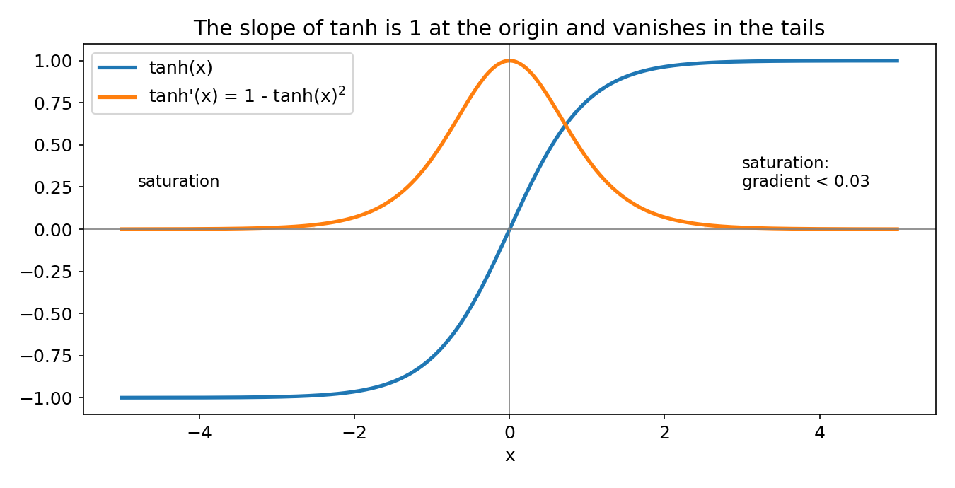
tanh and its derivative

The picture explains why deep tanh networks were hard to train. The slope is at most 1 (at x=0x = 0) and drops below 0.03 once ∣x∣>2.5|x| > 2.5. Backpropagation multiplies these factors layer after layer, so saturated units let almost no gradient through: the vanishing gradient problem that ReLU and careful initialisation later fixed.

4.2 The vectorised gradient

The maths. Let rn=y[n]−θ⊤X[n]r_n = y[n] - \theta^\top X[n] be the residual of sample nn. By the chain rule, ∇θ rn2=2rn ∇θrn=−2rnX[n]\nabla_\theta\, r_n^2 = 2r_n\,\nabla_\theta r_n = -2 r_n X[n]. Averaging over the samples,

∇θL=−2N∑n=0N−1rn X[n].\nabla_\theta L = -\frac{2}{N}\sum_{n=0}^{N-1} r_n\, X[n] .

In matrix form this is −2NX⊤(y−Xθ)-\frac{2}{N}X^\top(y - X\theta), but @ and .T are forbidden. That rule is the real exercise: we have to express both products with broadcasting and reductions.

  • XθX\theta is, for each row nn, ∑jX[n,j] θ[j]\sum_j X[n,j]\,\theta[j]. X * theta broadcasts theta (shape (d,)(d,)) over the NN rows, and np.sum(..., axis=1) sums each row. That gives the predictions, shape (N,)(N,).
  • X⊤rX^\top r is, for each column jj, ∑nX[n,j] rn\sum_n X[n,j]\, r_n. residual[:, None] has shape (N,1)(N,1), so X * residual[:, None] scales row nn by rnr_n, and np.mean(..., axis=0) averages down the rows, which already contains the 1/N1/N.
import numpy as np

def my_fun_derivative(X, y, theta):
    residual = y - np.sum(X * theta, axis=1)              # (N,)
    return -2.0 * np.mean(X * residual[:, None], axis=0)  # (d,)

It uses no loop, no @, no .T and no np.linalg, and nothing is imported besides NumPy. The output has shape (d,)(d,) as required. A one-line sanity check by hand: with N=d=1N = d = 1, X=2X = 2, y=3y = 3, θ=0.5\theta = 0.5, the residual is 3−1=23 - 1 = 2 and the gradient is −2⋅2⋅2=−8-2 \cdot 2 \cdot 2 = -8, which the function returns.

Common pitfalls.

  • Forgetting the factor 2, or the minus sign that comes from differentiating y−θ⊤Xy - \theta^\top X (the gradient then points uphill).
  • Writing X * residual without [:, None]: shapes (N,d)(N,d) and (N,)(N,) only broadcast if d=Nd = N, and then the result is silently wrong. Keep axes explicit.
  • np.dot or np.matmul are not literally @, but they are matrix products and break the spirit of the rule; the broadcasting version is the safe answer.

What to remember

  • tanh⁡′=1−tanh⁡2\tanh' = 1 - \tanh^2: the derivative is written in terms of the function's own output, which is exactly what backpropagation needs.
  • Saturating activations have tiny gradients in their tails: that is the root of vanishing gradients.
  • The MSE gradient is "minus twice the average of residual times input": −2NX⊤(y−Xθ)-\frac{2}{N}X^\top(y - X\theta).
  • Any matrix product can be rebuilt from broadcasting plus a sum over the shared axis. Thinking in terms of shapes, (N,d)×(d,)→(N,)(N,d) \times (d,) \to (N,), is the key skill.
  • Always check a hand-derived gradient against finite differences.
Code complet (solution.py)
"""USAAIO 2026 Round 1, Problem 4: derivative of tanh, and a loop-free MSE gradient in NumPy.

Rules of Part 4.2: only `import numpy as np`; no autograd, nothing from np.linalg, no `@`, no `.T`,
no loops.  We check both parts numerically against central finite differences.
"""
import numpy as np


def my_fun_derivative(X, y, theta):
    """Gradient of (1/N) * sum_n (y[n] - theta . X[n])^2 with respect to theta, shape (d,)."""
    residual = y - np.sum(X * theta, axis=1)            # (N,): theta broadcast along rows
    return -2.0 * np.mean(X * residual[:, None], axis=0)  # (d,): average of residual-weighted rows


# ------------------------------------------------------------------ checks (not part of the answer)
if __name__ == '__main__':
    rng = np.random.default_rng(0)

    # 4.1: d tanh / dx = 1 - tanh(x)^2 = 1 / cosh(x)^2
    x = np.linspace(-4, 4, 81); h = 1e-5
    fd = (np.tanh(x + h) - np.tanh(x - h)) / (2 * h)
    print('4.1 max |finite difference - (1 - tanh^2)| =', np.abs(fd - (1 - np.tanh(x) ** 2)).max())

    # 4.2: compare with finite differences and with the matrix formula -2/N X^T (y - X theta)
    N, d = 500, 7
    X, y, theta = rng.normal(size=(N, d)), rng.normal(size=N), rng.normal(size=d)
    loss = lambda t: np.mean((y - np.sum(X * t, axis=1)) ** 2)
    g = my_fun_derivative(X, y, theta)
    fd = np.array([(loss(theta + h * e) - loss(theta - h * e)) / (2 * h) for e in np.eye(d)])
    print('4.2 max |finite difference - ours| =', np.abs(fd - g).max())
    print('4.2 max |matrix formula   - ours| =', np.abs(-2 / N * X.T @ (y - X @ theta) - g).max())
    # edge case N = 1, d = 1
    print('4.2 N=d=1:', my_fun_derivative(np.array([[2.0]]), np.array([3.0]), np.array([0.5])),
          '(expected -2*2*(3-1) = -8)')