IOAI Training: Learn AI by solving problems

The problem in brief

A synthetic survey describes 98,490 people (age, city, profession or degree, pressure and satisfaction at work or at school, sleep, diet, financial stress, family history, suicidal thoughts) together with whether they report depression. You must predict depression for 42,210 other respondents, and the score is accuracy; the documentation of what you tried also counts. The notebook and data come from a third-party repository (github.com/teodora-dimitrova/Singapore-Team-Selection), which also contains the organisers' test labels and a coaches-only solution notebook. We did not open that notebook, and we used the test labels exactly once, after every choice had been made by cross-validation on the training set.

How you are scored

\text{accuracy} = \frac{1}{n}\sum_{i=1}^{n}\mathbf 1[\hat y_i = y_i] .

18.2 % of the training respondents are depressed, so predicting "no depression" for everyone already scores 81.8 %: that is the floor any model must beat. The statement gives no threshold.

First look at the data

The notebook warns that "data artifacts have been left in the synthetic dataset". Three structures matter.

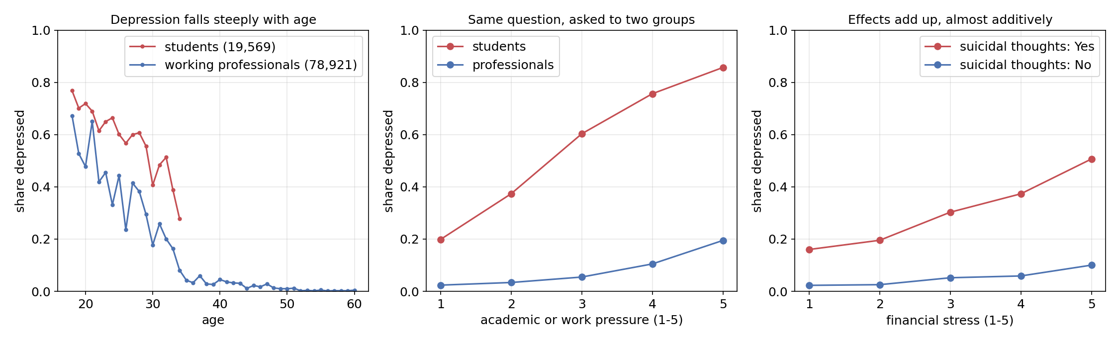
Two populations answer different questions. 19.9 % of respondents are students and the rest are working professionals. Students fill in Academic Pressure, CGPA and Study Satisfaction (missing for everyone else), professionals fill in Work Pressure and Job Satisfaction (missing for students). The 80 % "missing values" are not missing at random: they encode the group. The two populations are also very different: 58.5 % of students are depressed against 8.2 % of professionals.
Noise in the categories. Sleep Duration has 30 values, of which 4 are real ("Less than 5 hours", "5-6 hours", "7-8 hours", "More than 8 hours", each about 23,000 times) and 26 appear fewer than 10 times. Dietary Habits contains values such as "Pratham" or "Class 12" (a degree!). City, Profession and Degree have 85, 59 and 100 values, many of them single typos. Name is a random string, useless for prediction.
The signal is simple and strong. Depression falls steeply with age, rises with pressure in both groups, and rises with financial stress, roughly multiplying the odds; respondents who report suicidal thoughts are 5 to 8 times more often depressed at every level of financial stress.

Left: share of depressed respondents by age for students and professionals. Middle: share by pressure level, for the academic pressure of students and the work pressure of professionals. Right: suicidal thoughts and financial stress act together on the odds.

A first baseline

The notebook's template encodes every text column with an ordinal code, fills missing numbers with the median, and fits a decision tree with default settings. In 5-fold cross-validation it reaches 89.9 %. That is well above the 81.8 % floor, but the tree reaches 100 % on its own training data: with no depth limit, it grows a leaf for almost every respondent and memorises the noise. One unconstrained tree is a high-variance model.

The key idea

The data were generated from a fairly smooth, nearly additive rule (on the log-odds scale) of a few variables. Two consequences.

1. Clean, merged features make even a linear model excellent. Academic Pressure and Work Pressure are the same question asked to two groups, so we merge them into one pressure column, and likewise Study and Job Satisfaction into satisfaction; CGPA gets the value -1 for non-students, and a student flag keeps the group. Sleep and diet are mapped to numbers (4, 5.5, 7.5 and 9 hours; unhealthy, moderate, healthy as 0, 1, 2), turning the rare junk values into missing. City, Profession and Degree keep only categories seen at least 100 times, the rest become "other". With these 15 features, a logistic regression

\log\frac{P(\text{depressed})}{1 - P(\text{depressed})} = \beta_0 + \sum_j \beta_j x_j

(one-hot encoding for the three text columns, standardised numbers) reaches 93.7 % in cross-validation. The additive log-odds form is exactly the shape we saw in the plots: each factor multiplies the odds.

2. Averaging many trees fixes the variance. Gradient boosting (LightGBM: 600 shallow trees of 31 leaves, learning rate 0.03, at least 50 respondents per leaf, row and column subsampling) reaches 93.8 %. Interestingly, it reaches the same 93.8 % on the raw columns (without Name): trees split on "Academic Pressure is missing" as easily as on our student flag, so they do not need the engineering. The engineering matters for linear models, for robustness to the junk categories, and for interpretation. In LightGBM's gain importance, age alone accounts for 49 % of the splits' gain, then suicidal thoughts (13 %), profession (8 %) and pressure (7 %).

Since the two models make somewhat different errors (one is smooth and additive, the other piecewise constant), averaging their probabilities is a cheap ensemble: 93.8 % in cross-validation. We fixed this blend as the submission before computing any test score.

The full solution

Drop id and Name; build the 15 engineered features above, learning the frequent categories on the training set only.
Logistic regression (one-hot for City, Profession, Degree; median imputation and standardisation for the numbers).
LightGBM with native categorical handling for the three text columns.
Average the two predicted probabilities and threshold at 0.5.

X["pressure"] = d["Academic Pressure"].fillna(d["Work Pressure"])      # same question, two groups
X["satisfaction"] = d["Study Satisfaction"].fillna(d["Job Satisfaction"])
X["sleep"] = d["Sleep Duration"].map(SLEEP)                             # junk values -> NaN

The whole script, with cross-validation of every model, runs in about 25 seconds on a laptop.

Results

model	5-fold CV accuracy (train)	test accuracy
always "no depression"	81.8 %	81.9 %
decision tree, raw ordinal features (notebook template)	89.9 %
logistic regression, engineered features	93.7 %	94.0 %
LightGBM, raw columns	93.8 %
LightGBM, engineered features	93.8 %	94.0 %
blend of logistic regression and LightGBM (submitted)	93.8 %	94.1 %

The test labels were used only for the last column, after the submission was fixed. Cross-validation predicted the test accuracy within 0.3 points, which confirms that the training and test files come from the same distribution. The remaining 6 % of errors seem to be irreducible noise for these features (respondents whose answers look typical of the other class), which would explain why the logistic regression, the boosted trees and their blend all land within 0.1 point of each other.

What to remember

Missing values can be information. Here "missing" meant "this question was not asked to you"; merging parallel columns and keeping a group flag turns 80 % missingness into clean features.
Clean categories before modelling. Mapping ordered answers to numbers and folding rare typos into "other" protects linear models and makes the pipeline robust to unseen junk.
An unconstrained decision tree memorises. 100 % on training data, 90 % in cross-validation: limit its depth, or average many trees (forests, boosting).
When the signal is additive, logistic regression is competitive with boosting. Plot the target rate against each variable first; if each factor multiplies the odds, a linear model in log-odds is the right shape.
Fix the submission by cross-validation, then look at the test. Here CV and test agree within 0.3 points, which is the sign of an honest protocol.

"""Singapore IOAI 2025 selection test (ML): predict Depression from a synthetic mental-health survey.

Files from the task folder: train_IOAI.csv, test_IOAI.csv (and, for the final check only, the
organisers' test file with labels, saved here as test_labels.csv).
usage: python solution.py        -> 5-fold CV of every model, then test accuracy, writes submission.csv
"""
import os
import numpy as np, pandas as pd, lightgbm as lgb
from sklearn.linear_model import LogisticRegression
from sklearn.model_selection import StratifiedKFold
from sklearn.preprocessing import OrdinalEncoder, OneHotEncoder, StandardScaler
from sklearn.compose import ColumnTransformer
from sklearn.pipeline import make_pipeline
from sklearn.impute import SimpleImputer
from sklearn.tree import DecisionTreeClassifier

tr, te = pd.read_csv("train_IOAI.csv"), pd.read_csv("test_IOAI.csv")
y = tr.Depression.values
SLEEP = {"Less than 5 hours": 4, "5-6 hours": 5.5, "6-7 hours": 6.5, "7-8 hours": 7.5, "More than 8 hours": 9}
DIET = {"Unhealthy": 0, "Moderate": 1, "Healthy": 2}

def raw(d):
    """The notebook's preprocessing: all columns except id/target, ordinal codes for text."""
    return d.drop(columns=["id", "Depression"], errors="ignore")

def engineer(d, ref=tr):
    """Our features: merge the student / professional columns and clean the data artifacts."""
    X = pd.DataFrame(index=d.index)
    student = (d["Working Professional or Student"] == "Student").astype(int)
    X["student"] = student
    X["age"] = d.Age
    # Students answer Academic Pressure / Study Satisfaction, professionals Work Pressure / Job Satisfaction:
    # the same question asked to two groups, so merge them into one column each.
    X["pressure"] = d["Academic Pressure"].fillna(d["Work Pressure"])
    X["satisfaction"] = d["Study Satisfaction"].fillna(d["Job Satisfaction"])
    X["cgpa"] = d.CGPA.fillna(-1)                         # only students have a CGPA
    X["hours"] = d["Work/Study Hours"]
    X["financial"] = d["Financial Stress"]
    X["suicidal"] = (d["Have you ever had suicidal thoughts ?"] == "Yes").astype(int)
    X["family"] = (d["Family History of Mental Illness"] == "Yes").astype(int)
    X["male"] = (d.Gender == "Male").astype(int)
    # Sleep / diet: a few hundred typos and noise values ("Pratham", "Class 12") -> NaN
    X["sleep"] = d["Sleep Duration"].map(SLEEP)
    X["diet"] = d["Dietary Habits"].map(DIET)
    # High-cardinality text: keep categories seen at least 100 times in train, the rest -> "other"
    for c in ["City", "Profession", "Degree"]:
        common = ref[c].value_counts()
        common = set(common[common >= 100].index)
        X[c.lower()] = d[c].where(d[c].isin(common), "other").fillna("none")
    return X

CAT = ["city", "profession", "degree"]

def models():
    return {
        "decision tree, raw features (notebook)": ("raw", lambda: make_pipeline(
            ColumnTransformer([("num", SimpleImputer(strategy="median"), lambda X: X.select_dtypes("number").columns.tolist()),
                               ("cat", make_pipeline(SimpleImputer(strategy="constant", fill_value="missing"),
                                                     OrdinalEncoder(handle_unknown="use_encoded_value", unknown_value=-1)),
                                lambda X: X.select_dtypes("object").columns.tolist())]),
            DecisionTreeClassifier(random_state=42))),
        "logistic regression, engineered": ("eng", lambda: make_pipeline(
            ColumnTransformer([("num", make_pipeline(SimpleImputer(strategy="median"), StandardScaler()),
                                lambda X: [c for c in X.columns if c not in CAT]),
                               ("cat", OneHotEncoder(handle_unknown="ignore"), CAT)]),
            LogisticRegression(C=1.0, max_iter=3000))),
        "LightGBM, engineered": ("eng", lambda: lgb.LGBMClassifier(
            n_estimators=600, learning_rate=0.03, num_leaves=31, min_child_samples=50, subsample=0.8, subsample_freq=1,
            colsample_bytree=0.8, reg_lambda=1.0, n_jobs=2, verbose=-1)),
    }

def features(kind, d):
    if kind == "raw":
        return raw(d)
    X = engineer(d)
    for c in CAT:
        X[c] = X[c].astype("category")
    return X

def fit_predict(kind, make, Xa, ya, Xb):
    m = make()
    if kind == "eng" and isinstance(m, lgb.LGBMClassifier):
        m.fit(Xa, ya, categorical_feature=CAT)
    else:
        if kind == "eng":
            Xa, Xb = Xa.astype({c: str for c in CAT}), Xb.astype({c: str for c in CAT})
        m.fit(Xa, ya)
    return m.predict_proba(Xb)[:, 1]

if __name__ == "__main__":
    cv = StratifiedKFold(5, shuffle=True, random_state=0)
    oof = {}
    for name, (kind, make) in models().items():
        X = features(kind, tr)
        p = np.zeros(len(y))
        for a, b in cv.split(X, y):
            p[b] = fit_predict(kind, make, X.iloc[a], y[a], X.iloc[b])
        oof[name] = p
        print(f"{name:42s} CV accuracy {((p > 0.5) == y).mean():.4f}", flush=True)
    blend = (oof["logistic regression, engineered"] + oof["LightGBM, engineered"]) / 2
    print(f"{'blend LR + LightGBM':42s} CV accuracy {((blend > 0.5) == y).mean():.4f}")
    # Final: train on all training rows, predict the test set
    kind, make = models()["LightGBM, engineered"]
    p_lgb = fit_predict(kind, make, features(kind, tr), y, features(kind, te))
    kind, make = models()["logistic regression, engineered"]
    p_lr = fit_predict(kind, make, features(kind, tr), y, features(kind, te))
    pred = (((p_lgb + p_lr) / 2) > 0.5).astype(int)
    pd.DataFrame({"id": te.id, "Depression": pred}).to_csv("submission.csv", index=False)
    if os.path.exists("test_labels.csv"):  # organisers' labels: used once, after every choice was made
        gold = pd.read_csv("test_labels.csv").set_index("id").Depression.loc[te.id].values
        for nm, p in [("LightGBM", p_lgb), ("logistic regression", p_lr), ("blend (submitted)", (p_lgb + p_lr) / 2)]:
            print(f"test accuracy {nm}: {((p > 0.5) == gold).mean():.4f}")

Mental Health ML Task