IOAI Training: Learn AI by solving problems

The problem in brief

The story: after a (fictional) cyberattack, millions of Singapore public-housing (HDB) resale records lost one column, the storey range of the flat ("01 TO 03", "04 TO 06", up to "49 TO 51"). You get 105 000 intact records (real data.gov.sg transactions from 2017 to 2025: month, town, block, street, flat type and model, floor area, lease dates, resale price) and must recover the storey range of 104 460 damaged records. It is a 17-class classification problem on tabular data, scored by accuracy.

How you are scored

\text{accuracy} = \frac{1}{n}\sum_{i=1}^{n} \mathbb{1}\big[\hat y_i = y_i\big]

over the test records. The ground truth of the test set is public in the mirror we used, so we report the official test accuracy, after choosing everything on the same 80/20 split of the training set that the starter notebook uses. No threshold, baseline score or leaderboard was published; the reference points are the trivial baselines below.

First look at the data

Imbalanced, ordered classes. "04 TO 06" alone is 23 % of the records; above floor 18 the classes are rare (3 % in total for the 9 highest ranges). The classes are ordered: confusing floor 5 with floor 8 is a smaller mistake than with floor 35.
No leaks. Fewer than 0.3 % of test rows coincide with a training row on every feature, so you cannot just look the answers up.
The storey is priced in, but weakly in raw form. Across the whole dataset, price and storey have a Spearman correlation of only 0.25: a 5-room flat in a cheap town on floor 20 can cost less than a 3-room flat downtown on floor 2. Price is driven first by size, location and the age of the lease.

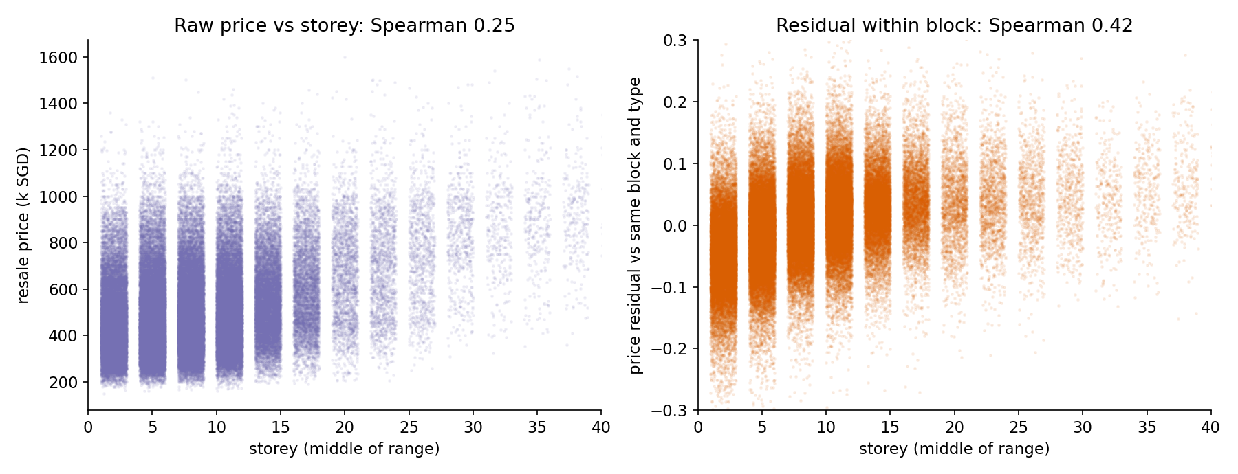
Left: resale price against storey for all training records, a weak trend (Spearman 0.25). Right: the price residual of each flat relative to flats of the same block and type, against storey: a much clearer upward trend (Spearman 0.42).

The right panel is the whole idea of this correction: compare each flat with its neighbours in the same block, and the storey effect appears.

A first baseline

baseline (validation = 20 % of train)	accuracy
always predict the most frequent range, "04 TO 06"	0.230
most frequent range of the same block in training	0.214
LightGBM 17-class classifier on the raw columns	0.249

A strong learner on the raw columns barely beats the constant guess. The raw table hides the signal: the model would have to learn, for each of the 9 550 blocks separately, what "expensive" means there.

The key idea

Write the log price of a flat as a sum of effects:

\log(\text{price}) \approx \underbrace{m(\text{month}, \text{type})}_{\text{market}} + \underbrace{\log(\text{area})}_{\text{size}} + \underbrace{b(\text{block})}_{\text{location, lease}} + \underbrace{s(\text{storey})}_{\text{what we want}} + \varepsilon .

Everything except $s$ can be estimated without labels, from the prices themselves:

Remove the market. HDB prices rose by roughly 50 % between 2017 and 2025. Subtract from the log price per square metre the median for the same month and flat type: we get an inflation-free price adj.
Remove the block. Subtract the mean adj of all flats of the same block and type (and also within the same block and year), and compute the percentile rank of the flat inside its block. What remains, res_bt, is mostly the storey effect plus noise.
Use the unlabelled rows too. These statistics need no storey label, so we compute them on training and test records together: a block's damaged records still tell us what its typical price is. This is legitimate (no label is touched) and doubles the number of comparables per block.

Then a second insight about the target: the classes are ordered, so treat it as regression. We regress the class index $0, \dots, 16$ with an L1 (absolute error) loss and round to the nearest class. Why L1? The constant minimising $\sum |y_i - c|$ is the median, and for an ordered target the median of the conditional distribution is the natural single guess. The loss also tells the model that missing by one range is much better than missing by five, information a 17-class cross-entropy throws away.

The full solution

Parse month into a month index, remaining_lease into months, build an address key block + street.
Price features (train and test together): log_ppsqm, adj, residuals and ranks within block, within block and type, within block, type and year, plus group sizes and spreads.
LightGBM regression, objective regression_l1, 600 trees, learning rate 0.05, 63 leaves, at least 40 records per leaf; predict, round, clip to $[0, 16]$ .

idx = d.groupby(["t", "ft"]).log_ppsqm.transform("median")        # market index
d["adj"] = d.log_ppsqm - idx                                        # inflation-free price
g = d.groupby(["addr", "ft"]).adj
d["res_bt"], d["rank_bt"] = d.adj - g.transform("mean"), g.rank(pct=True)

The most important features of the final model (by gain) are, in order, res_bt, the town, res_bty, the lease start year and rank_bt: the block-relative price is by far the strongest signal.

Results

approach	validation acc.	test acc.
most frequent class	0.230	0.229
block's most frequent class	0.214
LightGBM classifier, raw columns	0.249
LightGBM L1 regression, raw columns	0.279
hand rule: block's storey range scaled by the price rank in the block	0.303
LightGBM classifier, raw + block-relative price	0.280
+ out-of-fold "storeys seen in this block" statistics (classifier)	0.243
LightGBM L1 regression, raw + block-relative price (final)	0.323	0.328
same + out-of-fold block storey statistics	0.323
same + "comparable sales" (storeys of the closest-priced labelled flats in the block)	0.325

The final model is right on the exact range 32.8 % of the time on the official test set (against 22.9 % for the constant guess), and within one range 79.1 % of the time.

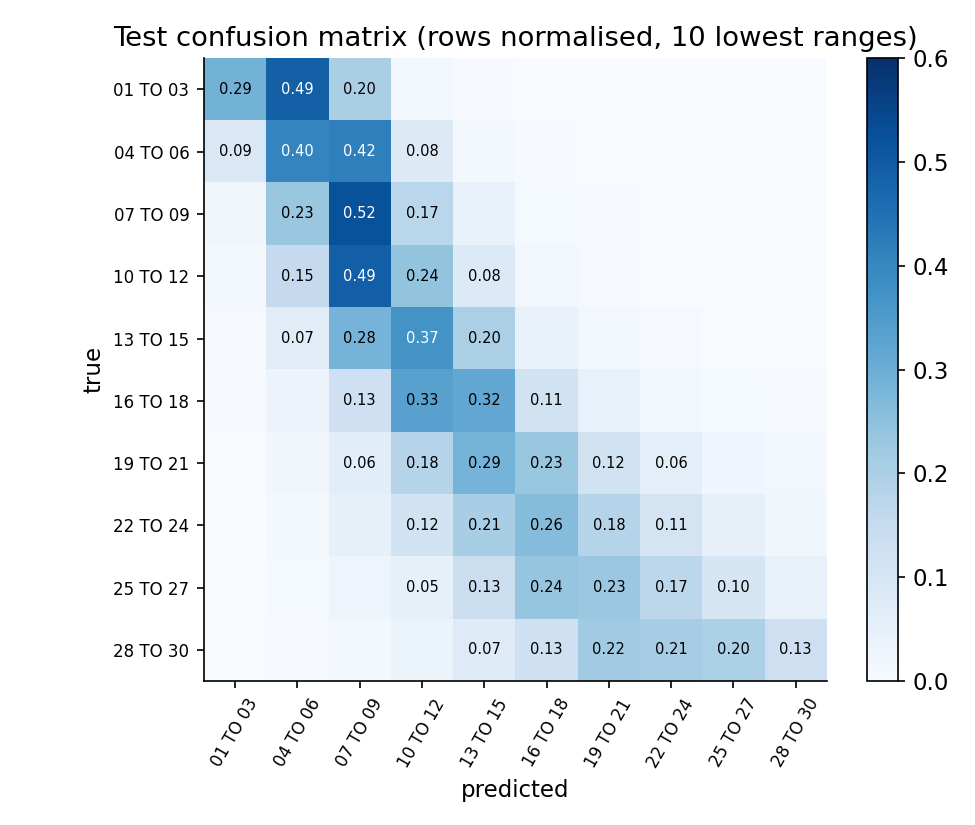
Row-normalised confusion matrix on the test set for the ten lowest storey ranges: the mass sits on the diagonal and its two neighbouring cells, with a visible pull toward the middle ranges 04 TO 06 and 07 TO 09.

What the failures teach:

Regression pulls toward the middle. Flats on floors 1 to 3 are predicted "04 TO 06" half of the time, and high floors are underestimated: when the evidence is weak, the conditional median sits near the bulk of the data. Tuning the rounding thresholds (instead of rounding at .5) is the obvious next step.
Out-of-fold target statistics did not help (and hurt the classifier). Blocks have only about 11 labelled sales each, so "which storeys exist in this block" is a noisy estimate, and the block-relative price already carries the useful part. Target encoding is not a free lunch on small groups.
Comparable sales (a kNN on price inside the block) added nothing over the residual features: gradient boosting had already extracted that information.
The ceiling is real. Within a block, price differences between floors are a few percent, comparable to the noise from renovation, view and negotiation (the right panel above shows heavy overlap between neighbouring floors). An exact-range accuracy around one third, with four out of five predictions within one range, is what the data allows with these features.

What to remember

Make the comparison explicit. Tree models do not easily compute "this flat versus its block"; residuals and ranks within a group (groupby().transform) hand them that signal directly.
Remove known trends before comparing (inflation here): a residual is only meaningful once the big effects are gone.
Unlabelled rows still carry information: group statistics computed on train plus test features use no labels and are fair game.
Ordered classes deserve an ordinal treatment. Regression with an L1 loss plus rounding beat a 17-class classifier by 4 points of accuracy here.
Report the honest ceiling and the near misses (within-one accuracy, confusion matrix): on noisy targets they say more than a single accuracy figure.

"""IOAI Singapore 2025 residential camp, ML challenge: recover the missing storey_range of HDB resale records.

Idea: the storey of a flat is not written anywhere, but it is *priced in*. Two flats of the same block,
same type, sold the same year differ in price mostly because of their floor. So we
  1. remove the market trend (month) and the size effect from the price,
  2. compare each flat with its neighbours in the same block (residual + percentile rank),
  3. treat the 17 storey ranges as an ORDERED target (regression with an L1 loss, then rounding),
and let gradient boosting combine these features.

Data: IOAI2025_ML_Challenge_trainset.csv / _testset.csv / testset_groundtruth.csv from
github.com/teodora-dimitrova/Singapore-Team-Selection ("IOAI 2025 Residential camp task/ ML_ResidentialCamp2025"),
saved as work/train.csv, work/test.csv, work/gt.csv.
Run: python solution.py
"""
import numpy as np, pandas as pd, lightgbm as lgb
from sklearn.model_selection import train_test_split
from sklearn.metrics import accuracy_score

SEED = 42
tr = pd.read_csv("work/train.csv", index_col=0)
te = pd.read_csv("work/test.csv", index_col=0)
gt = pd.read_csv("work/gt.csv", index_col=0)["storey_range"]
LABELS = sorted(tr.storey_range.unique())                  # "01 TO 03" ... "49 TO 51"
lab2i = {l: i for i, l in enumerate(LABELS)}

def base_features(df):
    d = pd.DataFrame(index=df.index)
    ym = df.month.str.split("-", expand=True).astype(int)
    d["t"] = (ym[0] - 2017) * 12 + ym[1] - 1               # months since Jan 2017
    rl = df.remaining_lease.str.extract(r"(\d+) years?(?: (\d+) months?)?").fillna(0).astype(int)
    d["lease_left"] = rl[0] * 12 + rl[1]
    d["area"] = df.floor_area_sqm
    d["lease_start"] = df.lease_commence_date
    d["log_price"] = np.log(df.resale_price)
    d["log_ppsqm"] = d.log_price - np.log(d.area)
    for c in ["town", "flat_type", "flat_model"]: d[c] = df[c].astype("category")
    d["addr"] = df.block.astype(str) + " " + df.street_name
    d["ft"] = df.flat_type
    return d

def price_features(d):
    """Unsupervised price statistics, computed on train+test features together (no labels used)."""
    # 1) market index: median log price per sqm per (month, flat type) -> remove inflation over 2017-2025
    idx = d.groupby(["t", "ft"]).log_ppsqm.transform("median")
    d["adj"] = d.log_ppsqm - idx
    # 2) compare with the same block (and same block + same type): residual and rank
    for key, name in [(["addr"], "b"), (["addr", "ft"], "bt")]:
        g = d.groupby(key).adj
        d[f"res_{name}"] = d.adj - g.transform("mean")
        d[f"rank_{name}"] = g.rank(pct=True)
        d[f"n_{name}"] = g.transform("size")
        d[f"std_{name}"] = g.transform("std")
    # 3) same block, nearby lease decay: older sales of the same block drift; use a +-12 month window
    d["year"] = d.t // 12
    g = d.groupby(["addr", "ft", "year"]).adj
    d["res_bty"] = d.adj - g.transform("mean"); d["rank_bty"] = g.rank(pct=True)
    return d

RAW = ["t", "lease_left", "area", "lease_start", "log_price", "town", "flat_type", "flat_model"]
PRICE = ["log_ppsqm", "adj", "res_b", "rank_b", "n_b", "std_b", "res_bt", "rank_bt", "n_bt", "std_bt",
         "res_bty", "rank_bty"]
FEATS = RAW + PRICE

def fit_predict(d_lab, y_lab, d_pred, rounds=600):
    """Storey ranges are ORDERED: regress the class index with an L1 loss, then round.
    The L1 loss aims at the conditional median, which is what rounding to one class needs;
    a wrong-by-one guess is penalised less than a wrong-by-five one during training."""
    params = dict(objective="regression_l1", learning_rate=0.05, num_leaves=63, min_data_in_leaf=40,
                  num_threads=2, verbose=-1, seed=SEED)
    m = lgb.train(params, lgb.Dataset(d_lab[FEATS], y_lab.values), rounds)
    return m, np.clip(np.round(m.predict(d_pred[FEATS])), 0, len(LABELS) - 1).astype(int)

if __name__ == "__main__":
    allX = pd.concat([tr.drop(columns="storey_range"), te])
    D = price_features(base_features(allX))
    y = tr.storey_range.map(lab2i)
    Dtr, Dte = D.loc[tr.index], D.loc[te.index]

    # ---- validation exactly as in the starter notebook: random 80/20 split of the train set
    i_tr, i_va = train_test_split(tr.index, test_size=0.2, random_state=42, shuffle=True)
    _, pred_va = fit_predict(Dtr.loc[i_tr], y.loc[i_tr], Dtr.loc[i_va])
    print("validation accuracy:", accuracy_score(y.loc[i_va], pred_va))
    print("validation within one range:", np.mean(np.abs(y.loc[i_va].values - pred_va) <= 1))

    # ---- final model on all labelled rows, scored once on the official ground truth
    model, pred_te = fit_predict(Dtr, y, Dte)
    out = pd.DataFrame({"storey_range": [LABELS[i] for i in pred_te]}, index=te.index)
    out.to_csv("work/predictions.csv")
    print("TEST accuracy:", accuracy_score(gt.loc[te.index], out.storey_range))
    imp = pd.Series(model.feature_importance("gain"), FEATS).sort_values(ascending=False)
    print(imp.head(15))

When Machine Learning meet Cybersecurity (HDB resale recovery)