IOAI Training: Learn AI by solving problems

The problem in brief

This selection test walks you through a standard image-classification pipeline on CIFAR-10 (50,000 training and 10,000 test images of 32x32 pixels, 10 classes). A warm-up section trains a plain multilayer perceptron. Question 1 asks you to fill in the missing pieces of a ResNet-18 recipe: two lines of data augmentation, the three-layer input stem of the network and the loss function, then train for 10 epochs. Question 2 is open: improve the accuracy with a deeper ResNet, hyperparameter tuning or dropout. CIFAR-10's test labels are public, so all numbers below are on the official test set; the notebook comes from a third-party repository (github.com/teodora-dimitrova/Singapore-Team-Selection), and we loaded CIFAR-10 from the Hugging Face mirror uoft-cs/cifar10 (identical images).

How you are scored

The notebook gives no marks or thresholds: the metric is simply the test accuracy, the fraction of the 10,000 test images classified correctly. The only reference points are in the text: the warm-up MLP "achieves ~35 %", and ResNet-18 should do "much better".

A word on method: like the notebook, we report accuracy on the test set after each epoch to draw learning curves. To choose hyperparameters honestly in a real contest you would hold out part of the training set; here the comparisons are coarse (several points apart) and we fixed the settings in advance rather than picking the best epoch.

First look: a bug in the warm-up

The warm-up MLP (3072 to 1024 to 512 to 512 to 10, ReLU, SGD with learning rate 0.001, batch 4, 2 epochs) hides a classic mistake. The training loop scales the inputs with inputs / 255.0, so the network learns on pixels in $[0, 1]$ , but the evaluation cell uses images / 255.0 * 2 - 1, pixels in $[-1, 1]$ . The test images are shifted and stretched compared with everything the network has seen.

warm-up MLP	test accuracy
evaluated as in the notebook, inputs in $[-1, 1]$	36.6 %
evaluated with the same scaling as training, $[0, 1]$	41.7 %

The notebook's "~35 %" is the buggy number; fixing one line is worth 5 points. The rule is general: every preprocessing step must be identical at training and test time, ideally written once in a shared function. The MLP's weakness itself is structural: by flattening the image, it throws away the fact that neighbouring pixels belong together, and must learn separately what a "cat ear" looks like at every position.

Question 1: completing the ResNet-18 recipe

Q1.1, data augmentation.

transforms.RandomCrop(32, padding=4),
transforms.RandomHorizontalFlip(),

The crop pads the image with 4 black pixels on each side and cuts a random 32x32 window: the object moves by up to 4 pixels. The flip mirrors half the images. Both produce new, plausible training images every epoch, so the network learns that a horse shifted or facing left is still a horse; that invariance reduces overfitting.

Q1.2, the stem.

nn.Conv2d(3, 64, kernel_size=3, stride=1, padding=1, bias=False),
nn.BatchNorm2d(64),
nn.ReLU(inplace=True),

This is the CIFAR version of ResNet: the ImageNet stem (7x7 convolution with stride 2 followed by max-pooling) would shrink a 32x32 image to 8x8 before the first residual block. With a 3x3 convolution at stride 1, layer1 works at 32x32 and the three stride-2 stages bring it to 4x4, which the final avg_pool2d(out, 4) averages into a 512-dimensional vector. bias=False because the BatchNorm that follows has its own shift.

Q1.3, the loss. criterion = nn.CrossEntropyLoss(). It applies log-softmax and the negative log-likelihood in one numerically stable operation. The warm-up's hand-made version, -torch.log(softmax(...)), computes the same quantity but can return -inf when a probability underflows to 0.

With the notebook's settings (SGD, learning rate 0.01, momentum 0.9, weight decay $5\times10^{-4}$ , batch 128, 10 epochs), ResNet-18 reaches 85.3 %, twice the MLP's accuracy.

Question 2: what actually improves it

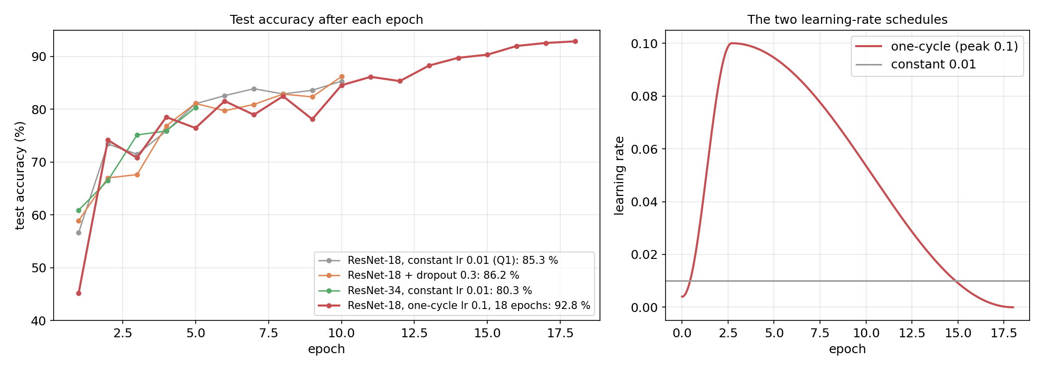
Left: test accuracy after each epoch for each variant. Right: the constant learning rate of Q1 against the one-cycle schedule that gave the best result.

The key observation is in the grey curve: with a constant learning rate, test accuracy keeps oscillating by one or two points from epoch to epoch (83.9 %, 82.9 %, 83.6 %, 85.3 %). The weights never settle: each SGD step with $\eta = 0.01$ adds noise of a fixed size, so the model bounces around the bottom of the loss valley instead of descending into it.

Hyperparameters: the learning-rate schedule is the big win. A one-cycle schedule raises the learning rate from 0.004 to 0.1 during the first 15 % of training, then lowers it along a cosine curve to almost zero (Nesterov momentum, same weight decay, batch 128, 18 epochs). The large learning rate early on explores fast and acts as a regulariser (big noisy steps cannot settle in sharp, overfitted minima); the decay at the end shrinks the noise so the weights converge into the minimum they have found. The red curve shows both phases: it is no better than the constant rate while the learning rate is high (78 to 85 % around epochs 5 to 10), then climbs steadily as it decays, to 92.8 %. The gain comes from the schedule, not only from the 8 extra epochs: the constant-rate curve only wandered between 82.9 and 85.3 % over its last 4 epochs.

Dropout. Dropout with $p = 0.3$ before the final linear layer gives 86.2 % after 10 epochs against 85.3 %. Given the epoch-to-epoch oscillations of about $\pm 1.5$ points, this difference is within the noise. That is expected: augmentation, weight decay and BatchNorm already regularise a convolutional network well, and after global average pooling only one 512-dimensional vector is left to drop. Dropout matters much more in large fully connected layers.

Deeper ResNet. ResNet-34 (3, 4, 6, 3 blocks instead of 2, 2, 2, 2) costs about twice as much per epoch (94 s against 47 to 62 s on our laptop GPU). Since a constant learning rate gives the same curve whatever the planned length, we can compare it after 5 epochs with ResNet-18's curve at epoch 5: 80.3 % against 81.0 %. Within a fixed compute budget, depth does not pay here: ResNet-18 already has the capacity to fit CIFAR-10 almost perfectly, and the bottleneck is optimisation (how long and how well we train), not model size. With a schedule and 100+ epochs, ResNet-34 and ResNet-50 do end up about 0.5 to 1 point above ResNet-18, but that takes hours.

The full solution

solution.py contains the whole pipeline: the data loading, the augmentation (crop and flip batched on the GPU, equivalent to the two torchvision transforms), the notebook's network with the three stem lines, an optional dropout layer and a configurable depth, and the training loop with either the notebook's constant learning rate or the one-cycle schedule.

opt = torch.optim.SGD(net.parameters(), lr=0.1, momentum=0.9, weight_decay=5e-4, nesterov=True)
sch = torch.optim.lr_scheduler.OneCycleLR(opt, 0.1, total_steps=epochs * 391, pct_start=0.15)
# ... call sch.step() after every optimizer step, not every epoch

Results

All on the official CIFAR-10 test set.

model	training	test accuracy
warm-up MLP, notebook's evaluation (scaling bug)	2 epochs, batch 4	36.6 %
warm-up MLP, consistent scaling	2 epochs, batch 4	41.7 %
ResNet-18 (Q1)	constant lr 0.01, 10 epochs	85.3 %
ResNet-18 + dropout 0.3	constant lr 0.01, 10 epochs	86.2 %
ResNet-18	constant lr 0.01, 5 epochs	81.0 %
ResNet-34	constant lr 0.01, 5 epochs	80.3 %
ResNet-18	one-cycle, peak lr 0.1, 18 epochs	92.8 %

Training times on an Apple laptop GPU shared with other jobs: about 1 minute per ResNet-18 epoch, 22 minutes for the final run.

What to remember

Preprocess train and test the same way. A scaling mismatch costs points silently and never raises an error; write the preprocessing once and reuse it.
Convolutions and augmentation encode what we know about images: local patterns, translation and mirror invariance. That is why a ResNet doubles the MLP's accuracy with fewer parameters.
The learning-rate schedule is often the most valuable hyperparameter. High rate to explore, decaying rate to converge: one-cycle or cosine schedules turned 85 % into 93 %.
Judge a change against the noise level. With a constant learning rate, the test accuracy jumps by $\pm 1.5$ points between epochs; a 1-point "improvement" from dropout is not evidence.
Under a compute budget, train better before training bigger. Depth helped nothing here, while the same compute spent on a proper schedule gave 7 points.

"""Singapore IOAI 2024 selection test (CV): CIFAR-10 with an MLP, ResNet-18 and improvements.

usage: python solution.py data          # CIFAR-10 from the HF mirror uoft-cs/cifar10 -> .npy
       python solution.py mlp           # warm-up MLP, with the notebook's normalisation bug and fixed
       python solution.py resnet <depth 18|34> <epochs> <schedule const|cosine> <lr> <dropout>
e.g.   python solution.py resnet 18 10 const 0.01 0     (Q1, the notebook's recipe)
       python solution.py resnet 18 20 cosine 0.1 0     (Q2 best)
"""
import io, json, sys, time
import numpy as np, torch, torch.nn as nn, torch.nn.functional as F
torch.set_num_threads(2); torch.manual_seed(0)
DEV = torch.device("mps" if torch.backends.mps.is_available() else "cpu")

def make_data():
    import pandas as pd
    from PIL import Image
    for s in ["train", "test"]:
        d = pd.read_parquet(f"https://huggingface.co/datasets/uoft-cs/cifar10/resolve/main/plain_text/{s}-00000-of-00001.parquet")
        np.save(f"{s}_x.npy", np.stack([np.asarray(Image.open(io.BytesIO(b["bytes"])).convert("RGB")) for b in d.img]))
        np.save(f"{s}_y.npy", d.label.values.astype(np.int64))

def load(scale="pm1"):
    """pm1: ToTensor + Normalize(0.5, 0.5) -> [-1, 1];  01: ToTensor only -> [0, 1]."""
    f = lambda x: torch.from_numpy(x).permute(0, 3, 1, 2).float() / 255
    X, Xt = f(np.load("train_x.npy")), f(np.load("test_x.npy"))
    if scale == "pm1":
        X, Xt = X * 2 - 1, Xt * 2 - 1
    return X, torch.from_numpy(np.load("train_y.npy")), Xt, torch.from_numpy(np.load("test_y.npy"))

def augment(x):  # Q1.1: RandomCrop(32, padding=4) + RandomHorizontalFlip, batched on the device
    n, ar = x.shape[0], torch.arange(32, device=x.device)
    i, j = torch.randint(0, 9, (n, 1), device=x.device), torch.randint(0, 9, (n, 1), device=x.device)
    out = F.pad(x, (4, 4, 4, 4))[torch.arange(n, device=x.device)[:, None, None, None], torch.arange(3, device=x.device)[None, :, None, None],
                                 (i + ar)[:, None, :, None], (j + ar)[:, None, None, :]]
    flip = torch.rand(n, device=x.device) < 0.5
    out[flip] = out[flip].flip(3)
    return out

class ResidualBlock(nn.Module):  # the notebook's block
    def __init__(s, cin, cout, stride=1):
        super().__init__()
        s.left = nn.Sequential(nn.Conv2d(cin, cout, 3, stride, 1, bias=False), nn.BatchNorm2d(cout), nn.ReLU(inplace=True),
                               nn.Conv2d(cout, cout, 3, 1, 1, bias=False), nn.BatchNorm2d(cout))
        s.shortcut = nn.Sequential()
        if stride != 1 or cin != cout:
            s.shortcut = nn.Sequential(nn.Conv2d(cin, cout, 1, stride, bias=False), nn.BatchNorm2d(cout))
    def forward(s, x):
        return F.relu(s.left(x) + s.shortcut(x))

class ResNet(nn.Module):
    def __init__(s, blocks=(2, 2, 2, 2), dropout=0.0, num_classes=10):
        super().__init__()
        s.inchannel = 64
        s.conv1 = nn.Sequential(nn.Conv2d(3, 64, kernel_size=3, stride=1, padding=1, bias=False),   # Q1.2 line 1
                                nn.BatchNorm2d(64),                                                # Q1.2 line 2
                                nn.ReLU(inplace=True))                                             # Q1.2 line 3
        s.layers = nn.Sequential(*[s.make_layer(c, n, st) for c, n, st in zip((64, 128, 256, 512), blocks, (1, 2, 2, 2))])
        s.drop = nn.Dropout(dropout)                                                              # Q2.3
        s.fc = nn.Linear(512, num_classes)
    def make_layer(s, channels, num_blocks, stride):
        layers = []
        for st in [stride] + [1] * (num_blocks - 1):
            layers.append(ResidualBlock(s.inchannel, channels, st)); s.inchannel = channels
        return nn.Sequential(*layers)
    def forward(s, x):
        out = F.avg_pool2d(s.layers(s.conv1(x)), 4).flatten(1)
        return s.fc(s.drop(out))

@torch.no_grad()
def accuracy(net, Xt, yt, bs=500):
    net.eval()
    pred = torch.cat([net(Xt[k:k + bs].to(DEV)).argmax(1).cpu() for k in range(0, len(Xt), bs)])
    return (pred == yt).float().mean().item() * 100

def mlp():
    """Warm-up: 4-layer MLP, batch 4, SGD lr 1e-3, 2 epochs (run on CPU: tiny batches are faster there)."""
    X, y, Xt, yt = load("01")
    net = nn.Sequential(nn.Flatten(), nn.Linear(3072, 1024), nn.ReLU(), nn.Linear(1024, 512), nn.ReLU(),
                        nn.Linear(512, 512), nn.ReLU(), nn.Linear(512, 10))
    opt = torch.optim.SGD(net.parameters(), lr=0.001, momentum=0.9)
    for _ in range(2):
        perm = torch.randperm(len(y))
        for k in range(0, len(y), 4):
            b = perm[k:k + 4]
            loss = F.cross_entropy(net(X[b]), y[b]); opt.zero_grad(); loss.backward(); opt.step()
    with torch.no_grad():
        acc = lambda Z: (net(Z).argmax(1) == yt).float().mean().item() * 100
        print(f"MLP, test inputs scaled like training ([0,1]): {acc(Xt):.2f} %")
        print(f"MLP, test inputs scaled to [-1,1] as in the notebook's evaluation cell: {acc(Xt * 2 - 1):.2f} %")

def resnet(depth, epochs, schedule, lr, dropout):
    X, y, Xt, yt = load("pm1")
    blocks = {18: (2, 2, 2, 2), 34: (3, 4, 6, 3)}[depth]
    net = ResNet(blocks, dropout).to(DEV)
    criterion = nn.CrossEntropyLoss()                                                              # Q1.3
    opt = torch.optim.SGD(net.parameters(), lr=lr, momentum=0.9, weight_decay=5e-4, nesterov=schedule == "cosine")
    steps = epochs * ((len(y) + 127) // 128)
    sch = torch.optim.lr_scheduler.OneCycleLR(opt, lr, total_steps=steps, pct_start=0.15) if schedule == "cosine" else None
    curve, t0 = [], time.time()
    for ep in range(epochs):
        net.train()
        perm = torch.randperm(len(y))
        for k in range(0, len(y), 128):
            b = perm[k:k + 128]
            loss = criterion(net(augment(X[b].to(DEV))), y[b].to(DEV))
            opt.zero_grad(); loss.backward(); opt.step()
            if sch: sch.step()
        curve.append(accuracy(net, Xt, yt))
        print(f"epoch {ep + 1}: loss {loss.item():.3f}, test acc {curve[-1]:.2f} %, {time.time() - t0:.0f}s", flush=True)
    tag = f"r{depth}_{epochs}ep_{schedule}_lr{lr}_do{dropout}"
    json.dump({"curve": curve, "minutes": (time.time() - t0) / 60}, open(f"curve_{tag}.json", "w"))
    print(f"{tag}: final test accuracy {curve[-1]:.2f} %")

if __name__ == "__main__":
    cmd = sys.argv[1]
    if cmd == "data": make_data()
    elif cmd == "mlp": mlp()
    else: resnet(int(sys.argv[2]), int(sys.argv[3]), sys.argv[4], float(sys.argv[5]), float(sys.argv[6]))

Image Classification on CIFAR-10 via ResNet