IOAI Training: Learn AI by solving problems

The problem in brief

For a given place, you see five days of daily weather: minimum, average and maximum temperature, precipitation, snowfall, wind direction and speed, peak gust, pressure and sunshine. Many of these values are missing. You must say which of 36 extreme-weather categories will occur on the following day. The training file has 182 757 rows, and each row carries one label: an event type from 0 to 35, or -1 when nothing happened (16.6 % of rows). You print 36 zeros and ones for each of the 59 192 test rows. External data is forbidden. This is from the Swedish AI Olympiad qualifier 2025 (by Arvid Kristoffersson and Theodor Beskow).

The test labels are hidden, so we score on a held-out 20 % of the training data, split in the same way as the real test (see below).

How you are scored

For each row and each of the 36 categories, a false alarm costs 3.5 and a missed event costs 140. With $\bar p$ the average penalty per row,

\text{Points} = \max\Big(0, \min\Big(100,\ 101 - \Big(\frac{130}{130 - \bar p}\Big)^2\Big)\Big), \quad 0 \text{ if } \bar p \ge 130 .

Our reading: each test row, like each training row, has one true category, or none. The statement also warns that the scoring "may be adjusted during the competition", so absolute numbers on Kattis may differ from ours.

What to aim for. No threshold is given. On Kattis nobody scored 100, and the best scores are 94.4, 93.6 and 90.1.

First look at the data

Several events per day. The same weather row can appear several times with different labels: the same place and day produced several events (and identical rows with the same label are frequent too). 11 832 distinct weather rows carry more than one event type.
The test is split by weather row, not by line: only 0.08 % of test rows have weather identical to a training row. So our validation must hold out whole groups of identical rows. A random line split would let the model see the same day with another label.
Missing values: snowfall is missing in 72 % of rows, gust and sunshine in 99 %. Gradient boosting handles NaN natively.
Imbalance: the 4 most frequent events cover 36 % of rows, and the rarest has 309 rows.

A first baseline

On the held-out groups:

rule	penalty	points
all zeros (`baseline2.py`)	117.0	0.5
all ones	123.1	0
random bits (`baseline.py`), expected value	120.1	0

All zeros misses every event, and with a 140-point penalty per miss that is fatal.

The key idea

Turn the costs into a threshold. For one category $k$ on one row, let $p_k$ be the probability that this row's event is $k$ . Answering 1 costs 3.5 if the event is not $k$ . Answering 0 costs 140 if it is. The expected costs are $3.5(1 - p_k)$ and $140\,p_k$ , so answer 1 exactly when

140\, p_k > 3.5\,(1 - p_k) \iff p_k > \frac{3.5}{143.5} \approx 0.0244 .

The 36 decisions are independent, so this rule is optimal for each of them separately. Two consequences follow.

Even with no model at all, you should flag every category whose overall frequency exceeds 2.44 %. That is 12 categories, and it already gives penalty 68.9, 96.5 points: better than every Kattis score. You pay 3.5 for each of the dozen flags, but you rarely miss the common events.
With a model, all that matters is calibrated probabilities. You do not tune a threshold, you derive it. A multiclass classifier with 37 outputs (including "nothing") trained with log-loss gives calibrated probabilities $p_k$ , and it shrinks the flag list for each row to the categories that are plausible for this weather.

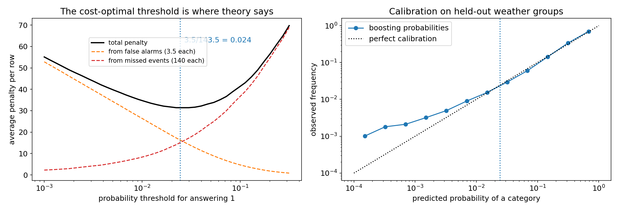
Penalty against threshold, and calibration of the probabilities

The left panel confirms the theory on held-out data: the penalty curve has its minimum at 0.026, right next to the predicted 0.0244. There, false alarms and missed events cost about the same. The right panel shows why: the boosted probabilities are well calibrated around the threshold (observed frequency equals predicted probability). They are only over-confident for categories they consider very unlikely (below 0.5 %), which are far below the threshold anyway.

The full solution

Features: the 50 raw columns, plus five summaries for each of the 10 variables: 5-day mean, 5-day maximum, last-day change (day 5 minus day 4), trend (day 5 minus day 1) and number of missing days. Also the sine and cosine of the last day's wind direction, since a direction is an angle.
HistGradientBoostingClassifier over the 37 classes: learning rate 0.05, up to 600 rounds, 31 leaves, at least 40 rows per leaf, L2 regularisation 1. Early stopping on an internal 10 % split never triggered.
Flag every category with $p_k > 3.5/143.5$ . That is 5.4 categories per row on average, and 87 % of events are caught.
For Kattis, the 36 bits of each row are packed into 5 bytes, compressed and printed by a small program (154 KiB). It works like the provided baseline2.py, which is itself 4.3 MB, so this problem accepts large sources. On the test rows the final model flags 6.8 categories per row on average (5.4 on our validation rows), a hint that the test days are somewhat more uncertain or that the model trained on all the data spreads its probabilities a little more.

Results

On 20 % of the weather groups held out from training (the test labels are private).

approach	penalty	points
all zeros	117.0	0.5
all ones	123.1	0
flag the 12 categories whose frequency exceeds 2.44 %	68.9	96.5
boosting on raw columns (stopped early after 50 rounds), threshold 0.0244	42.0	98.8
same, plus the number of identical rows in the file as a feature	43.3	98.8
boosting with 5-day summaries, 600 rounds, threshold 0.0244 (final)	31.3	99.3

Moving the threshold between 0.02 and 0.035 changes the penalty by less than 0.5, so the result does not depend on fine-tuning. One idea that did not help: counting how many times a weather row appears (a busy day often has several events) left the score unchanged, so we dropped it.

What to remember

With asymmetric costs, derive the decision threshold from them: answer 1 when $p > c_\text{FP}/(c_\text{FP} + c_\text{FN})$ . Here that is 0.024, far from 0.5.
That reduces the job to estimating calibrated probabilities. Log-loss models (logistic regression, boosting) give them. Check calibration on held-out data.
A no-model rule using only class frequencies can already be strong under such costs: always check it.
Split validation data the way the test was split. Here, identical weather rows had to stay together.
Boosting deals with missing values on its own. Summary features (means, changes, trends) help it see a 5-day pattern.

"""SAIO Windchill: from 5 days of weather, flag which of 36 extreme-weather types will occur.

Cost of a wrong 1 = 3.5, cost of a missed event = 140, so with calibrated probabilities p_k
the expected-cost-optimal rule is: answer 1 for category k  <=>  140 p_k > 3.5 (1 - p_k)
<=> p_k > 3.5 / 143.5 = 0.0244.  No threshold tuning needed: only good probabilities.
Probabilities: one multiclass gradient-boosting model over 37 classes (-1 = nothing happens)
on the raw columns + per-variable 5-day summaries (mean, max, last-day change, trend, #missing).
Training rows that share identical weather (same place and day, several events) are kept
together when splitting, as in the hidden test (only 0.08 % of test rows share weather with train).
  python3 solution.py --validate   # group hold-out (20 % of weather groups)
  python3 solution.py              # fit on all training rows, write submission.py for Kattis
Run from the folder holding trainingdata.csv and testdata.csv.
"""
import sys, zlib, base64, warnings, numpy as np, pandas as pd
from sklearn.ensemble import HistGradientBoostingClassifier
warnings.filterwarnings('ignore')
THR = 3.5 / (3.5 + 140)
VARS = ['tavg', 'tmin', 'tmax', 'prcp', 'snow', 'wdir', 'wspd', 'wpgt', 'pres', 'tsun']


def features(d, cols):
    out = d[cols].copy()
    for v in VARS:
        A = d[[f'day{i}{v}' for i in range(1, 6)]].values
        out[v + '_mean'] = np.nanmean(A, 1); out[v + '_max'] = np.nanmax(A, 1)
        out[v + '_d54'] = A[:, 4] - A[:, 3]; out[v + '_d51'] = A[:, 4] - A[:, 0]
        out[v + '_nan'] = np.isnan(A).sum(1)
    w = np.radians(d['day5wdir'].values); out['wsin5'], out['wcos5'] = np.sin(w), np.cos(w)
    return out.values


def penalty(P, y):
    """Average penalty of 0/1 predictions P (n, 36) against single labels y in {-1..35}."""
    pen = 3.5 * P.sum(1)
    idx = np.where(y >= 0)[0]
    pen[idx] += np.where(P[idx, y[idx]] == 1, -3.5, 140.0)
    return pen.mean()


def points(p):
    return 0.0 if p >= 130 else max(0.0, min(100.0, 101 - (130 / (130 - p)) ** 2))


def fit_proba(X, y, Xq):
    h = HistGradientBoostingClassifier(max_iter=600, learning_rate=0.05, max_leaf_nodes=31,
                                       l2_regularization=1.0, min_samples_leaf=40, early_stopping=True,
                                       validation_fraction=0.1, n_iter_no_change=30, random_state=0).fit(X, y)
    pr = h.predict_proba(Xq); cls = list(h.classes_)
    return np.stack([pr[:, cls.index(c)] if c in cls else np.zeros(len(Xq)) for c in range(36)], 1)


if __name__ == '__main__':
    tr = pd.read_csv('trainingdata.csv'); te = pd.read_csv('testdata.csv'); cols = list(te.columns)
    y = tr.EVENT_TYPE.values; X = features(tr, cols)
    if '--validate' in sys.argv:
        g = pd.util.hash_pandas_object(tr[cols].round(4), index=False).values   # one id per weather row
        held = set(np.random.default_rng(0).choice(np.unique(g), int(0.2 * len(np.unique(g))), replace=False))
        va = np.isin(g, list(held)); yv = y[va]
        prior = np.array([(y[~va] == c).mean() for c in range(36)])
        print('all zeros      : penalty %.2f, points %.2f' % (penalty(np.zeros((va.sum(), 36)), yv), points(penalty(np.zeros((va.sum(), 36)), yv))))
        Pp = np.tile(prior > THR, (va.sum(), 1)).astype(int)
        print('prior > %.4f : penalty %.2f, points %.2f' % (THR, penalty(Pp, yv), points(penalty(Pp, yv))))
        Pk = fit_proba(X[~va], y[~va], X[va]); P = (Pk > THR).astype(int)
        print('boosting       : penalty %.2f, points %.2f, %.1f categories flagged per row'
              % (penalty(P, yv), points(penalty(P, yv)), P.sum(1).mean()))
    else:
        P = (fit_proba(X, y, features(te, cols)) > THR).astype(np.uint8)
        blob = base64.b85encode(zlib.compress(np.packbits(P, axis=1).tobytes(), 9)).decode()
        open('submission.py', 'w').write(
            'import zlib,base64\nB=zlib.decompress(base64.b85decode(%r))\n'
            'for i in range(0,len(B),5):\n'
            '    bits="".join(format(c,"08b") for c in B[i:i+5])[:36]\n'
            '    print(" ".join(bits))\n' % blob)
        print('wrote submission.py,', len(blob) // 1024, 'KiB; mean categories flagged', P.sum(1).mean())