The problem in brief
You get one million German train arrivals (July 2024 to January 2026, open data from Deutsche Bahn) with the station (anonymised as a number from 0 to 99), the scheduled arrival time and the delay in minutes. For 100 000 more arrivals from the same period you only know the station and the time, and you must predict the delay (an integer, possibly negative: trains can be early). There is no public/private split and only 8 submissions are allowed, so all model selection has to happen on your own validation.
How you are scored
The metric is the mean squared error , mapped to points with a base of 90 and a best of 80:
Predicting the overall mean gives about 91 (the variance of the delays), so 90 is essentially "the constant", and 80 means explaining 11 % of the variance. We hold out a random 10 % of the training rows as validation, which mimics the test (random arrivals from the same period). On our validation split the constant gives 87.15, a bit lower than 91 by chance: a few extreme delays move the MSE of 100 000 rows by several units, so we compare relative gains rather than absolute numbers.
First look at the data
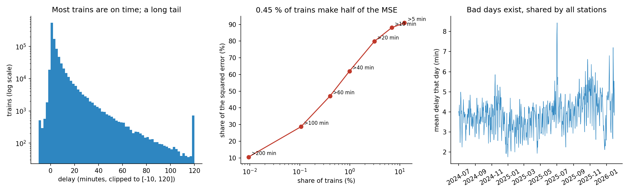
- The median delay is 1 minute, 90 % of trains are less than 10 minutes late, but the tail is long (1 % beyond 43 minutes, the maximum 521).
- The metric is dominated by rare disasters. Trains more than an hour off the mean are 0.45 % of the rows but make 49 % of the squared error. A model can only reduce the error where the big delays are somewhat predictable.
- There are a few absurd values around minutes: an arrival recorded just after midnight for a train scheduled just before, a clock wrap-around (24 h = 1440 min). They are noise for any model.
- Some days are much worse than others for the whole network (right panel), and stations differ in their average delay. Test rows are random arrivals from the same 19 months, so the test contains the same bad days as the training set: the date is a legitimate and very informative feature here, because it identifies the day's weather, strike or incident.
A first baseline
The organisers' notebook predicts 0 everywhere (worse than the mean, since the mean delay is 3.9 minutes). Predicting the training mean gives 87.15 on our validation split. Simple group means, smoothed toward the global mean, show which information matters (validation MSE):
| group mean by | MSE |
|---|---|
| nothing (constant) | 87.15 |
| weekday | 86.99 |
| hour of the day | 86.59 |
| calendar day | 86.47 |
| station and calendar day | 85.33 |
| station | 84.47 |
| station and hour of the day | 83.14 |
Station identity and its daily rhythm are the strongest signals; the calendar day adds information too, but each of these explains only a few percent.
The key idea
The delay is a sum of effects that interact: a given station is bad at 17:00 on weekdays, a storm on one day hurts some regions more, a strike hits every station. Group means can capture one combination at a time; gradient-boosted trees learn all the useful combinations from the raw features at once. A tree splits on, for example, "station in this set, and minute of the day between 16:30 and 18:45, and day index in this range", and boosting adds hundreds of such trees, each one correcting the residuals of the previous ones.
Two details matter because the metric is MSE.
- Predict the mean, not the median. With a squared loss the best constant per situation is the conditional mean. Delays are skewed, so the mean (3.9) sits well above the median (1): an "intuitive" median-based prediction would lose points.
- Tame the outliers in training, not in the predictions. We clip the training targets to minutes, so the clock wrap-arounds and the few extreme values cannot distort the fit. This barely changes the conditional means elsewhere (MSE 81.37 with clipping versus 81.45 without, within noise), and it protects the model against fitting noise.
The full solution
- Features: station (as a categorical variable), hour, minute of the day, weekday and day index since 1 July 2024.
- LightGBM, squared loss: 600 trees, learning rate 0.03, 63 leaves, at least 200 trains per leaf (a strong regulariser: with so much noise, a leaf must average many trains), row and column subsampling 0.8, targets clipped to .
- Fit on all training rows, predict the test rows, round to integers (rounding adds at most to the MSE on average).
m = lgb.LGBMRegressor(n_estimators=600, learning_rate=0.03, num_leaves=63,
                      min_child_samples=200, subsample=0.8, subsample_freq=1,
                      colsample_bytree=0.8)
m.fit(features(train), np.clip(y, -30, 150), categorical_feature=["station"])
Results
Validation MSE on a random 10 % of the training rows (the test labels are private):
| approach | validation MSE | gain vs constant |
|---|---|---|
| predict 0 (organisers' notebook) | about 102 | worse |
| constant mean | 87.15 | 0 % |
| smoothed mean by station and hour of the day | 83.14 | 4.6 % |
| LightGBM on 5 raw features (final) | 81.45 | 6.5 % |
| LightGBM + 7 out-of-fold target encodings (station-day, day-hour...) | 81.47 | 6.5 % |
| LightGBM + local windows (mean delay at the same station within 15 min to 6 h, and network-wide within 10 to 30 min) | 81.70 | 6.3 % |
If the same 6.5 % relative gain holds on the test set, whose constant error is about 90 to 91, our MSE would be about 84 to 85, which is roughly 55 to 60 points: an estimate, not a measured score.
The two failed rows are instructive. Hand-made encodings of "how late were the trains at this station that day" seemed promising, but the trees already found the same information from the raw day index and station, so the engineered features added nothing. The local time windows were even slightly worse: with only one million trains spread over 100 stations and 580 days, a station sees about 17 arrivals a day in the data, and the delay of a train 30 minutes earlier says little about the next one. The remaining error is mostly the large, unpredictable delays: half of the squared error comes from 0.45 % of the trains, and nothing in "station + scheduled time" announces them.
What to remember
- Find out where the squared error lives. When 0.45 % of the rows make half of the MSE, expect modest gains and focus on calibrating the mean, not on the typical case.
- Under MSE, predict conditional means: skewed targets make the mean very different from the median.
- Time can be a feature when train and test share the same period. A random split across the same days lets the model learn "bad days"; with a future test period this would be leakage-free but useless.
- Gradient boosting learns interactions (station x time of day x day) that one-at-a-time group means cannot.
- Check that feature engineering adds information, not just a new view of features the model already has; and with only 8 submissions, trust a clean validation split.