IOAI Training: Learn AI by solving problems

The problem in brief

A journal has been caught publishing a nonsense paper produced by an old automatic paper generator, the kind that strings together grammatical but meaningless computer-science sentences ("we disconfirm that the Turing machine and Smalltalk are largely incompatible"). Given the plain text of a paper, your program must print "Fake" or "Real". You get 10 generated papers and 50 real ones (arXiv papers in physics, mathematics and computer science, converted to text) as examples, and the hidden test papers are "comparable". It is from the Swedish AI Olympiad final 2025 (by Joshua Andersson and Rasmus Hulthe). Your program runs on Kattis on each paper, with a 1-second limit.

The test papers are hidden, so we evaluate by leave-one-out on the 60 examples: every fake paper is judged by a detector built without it.

How you are scored

With $TP$ the fraction of fake papers caught and $TN$ the fraction of real papers recognised as real,

\text{Score} = 100 \cdot TP \cdot TN^{2.5}.

The exponent punishes false accusations: missing one fake out of 10 costs 10 %, but wrongly flagging 1 real paper out of 50 costs $1 - 0.98^{2.5} \approx 5\%$ , and flagging 5 of them costs 23 %. The provided baseline answers "Fake" every time, so $TN = 0$ and it scores 0.

What to aim for. 100. The Kattis statistics show four full solves, then 84.2 and 84.1.

First look at the data

The fake papers are 9 500 to 12 500 characters long. The real ones range from 6 500 to 90 000. Length alone ("short means fake") gives at best $TP = 1$ , $TN = 0.72$ , which scores 44.
The fake papers read like a single author with a tiny vocabulary: "epistemologies", "our heuristic", "the Internet", "Smalltalk", "red-black trees", "we confirm that...". They also always have the same section skeleton (Introduction, Related Work, Implementation, Evaluation, Conclusion). The real papers cover every field, with formulas, names and domain jargon.
All 10 fakes put together use only 2 180 distinct words. That is the fingerprint of a grammar-based generator: it fills in templates from fixed word lists, so its outputs keep recycling the same words and, above all, the same word pairs.

A first baseline

A text classifier works out of the box. TF-IDF features plus logistic regression (balanced class weights), evaluated by leave-one-out, separates all 60 papers. The fakes get a probability of 0.89 to 0.93 and the most suspicious real paper 0.15, so the score is 100. But with 10 positive examples, a 600-dimensional linear model learnt from them is a black box whose behaviour on a new kind of real paper (a computer-science systems paper, say) is hard to predict. We want a rule whose safety margin we can measure and explain.

The key idea

A generator with a closed vocabulary reuses its own phrases. Collect every pair of consecutive words (bigram) that occurs in the known fake papers, about 8 100 of them. For any paper, measure its bigram coverage:

c(\text{paper}) = \frac{\#\{\text{bigrams of the paper that appear in a fake paper}\}}{\#\{\text{bigrams of the paper}\}} .

A generated paper is built from the same templates and word lists, so most of its word pairs have been seen before. A real paper only shares the generic ones ("of the", "in this", "we show"). Why bigrams rather than single words? Individual words are shared widely: even real papers have 56 % to 76 % of their words in the fake vocabulary, against 93 % to 96 % for fakes. Pairs are far more specific to the generator's templates, and the gap widens from a factor 1.2 to a factor 3.

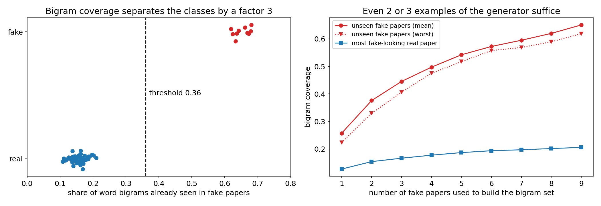
Bigram coverage of fake and real papers, and how many examples it needs

With leave-one-out (each fake paper measured against the bigrams of the 9 others):

fake papers: $c$ between 0.619 and 0.680;
real papers: $c$ between 0.108 and 0.209.

We put the threshold at the geometric middle of the gap, $\sqrt{0.619 \times 0.209} \approx 0.36$ . That leaves a safety factor of about 1.7 on each side.

Does it generalise? The right panel builds the bigram set from only $k$ of the fake papers and measures the coverage of the unseen ones. With $k = 2$ , the worst unseen fake still has 0.33 against 0.15 for the most fake-looking real paper. Coverage of new fakes grows steadily with $k$ , while real papers barely move. With all 10 fakes, which is what the submission uses, a new generated paper should land above 0.6, far from the threshold. This is the main argument that the hidden tests will behave the same way.

The full solution

Lower-case the text and keep runs of letters as words (the PDF-to-text conversion leaves hyphenations and stray numbers, which do no harm).
Build the set of word bigrams of the 10 fake papers.
Compute the coverage $c$ of the input paper and answer "Fake" if $c > 0.36$ .
For Kattis, the bigram set is zlib-compressed and base85-encoded inside a 40 KiB program. The whole computation is a single pass over the words, well under the 1-second limit even for a 300 000-character paper.

w = re.findall(r'[a-z]+', input().lower())
b = [w[i] + ' ' + w[i + 1] for i in range(len(w) - 1)]
print('Fake' if sum(x in K for x in b) / max(1, len(b)) > 0.36 else 'Real')

Results

Leave-one-out on the 60 example papers (the Kattis test papers are hidden).

approach	TP	TN	score
always "Fake" (baseline.py)	1.00	0.00	0
"Fake" if shorter than 13 000 characters	1.00	0.72	44
word coverage (any threshold between 0.76 and 0.93)	1.00	1.00	100
TF-IDF + logistic regression	1.00	1.00	100
bigram coverage $> 0.36$ (final)	1.00	1.00	100

Several methods reach 100 here. We chose bigram coverage because it has the widest, best-understood margin (a factor 3), it degrades gracefully when fewer examples of the generator are available, and it is one line of logic.

What to remember

When text comes from a template generator, its closed vocabulary is its signature. Measure how much of a document is made of "already seen" pieces.
Word pairs (n-grams) are much more specific than single words.
With an asymmetric score ( $TN^{2.5}$ ), place the threshold to maximise the margin on the costly side, and check that margin rather than just the accuracy.
With tiny data, evaluate by leave-one-out and stress-test generalisation by shrinking the training set, as in the right panel.
Prefer a simple rule you can reason about over a black box that happens to be perfect on 60 examples.

"""SAIO Nonsense (struntprat): tell SCIgen-style generated papers from real arXiv papers.

Idea: an old grammar-based generator reuses a small closed vocabulary and stock phrases.
Measure the share of a paper's word bigrams that also appear in the known fake papers
("bigram coverage"). Fakes reuse the generator's phrases (> 0.6), real papers almost never
(< 0.21). We evaluate with leave-one-out (a fake paper never sees its own bigrams), set the
threshold at the geometric middle of the gap, and write a Kattis program embedding the bigram set.
  data: work/fake/*.txt, work/real/*.txt (problem attachments)     python3 solution.py
"""
import glob, re, zlib, base64, numpy as np, matplotlib
matplotlib.use('Agg'); import matplotlib.pyplot as plt

tok = lambda s: re.findall(r'[a-z]+', s.lower())
bigrams = lambda w: list(zip(w, w[1:]))
fakes = [tok(open(f, errors='ignore').read()) for f in sorted(glob.glob('work/fake/*'))]
reals = [tok(open(f, errors='ignore').read()) for f in sorted(glob.glob('work/real/*'))]


def coverage(doc, known):
    b = bigrams(doc)
    return sum(x in known for x in b) / max(1, len(b))


# leave-one-out for fakes, all fakes for reals (reals never contribute to the bigram set)
cov_fake = [coverage(d, {b for j, o in enumerate(fakes) if j != i for b in bigrams(o)}) for i, d in enumerate(fakes)]
known = {b for d in fakes for b in bigrams(d)}
cov_real = [coverage(d, known) for d in reals]
thr = float(np.sqrt(min(cov_fake) * max(cov_real)))              # geometric middle of the gap
tp = np.mean(np.array(cov_fake) > thr); tn = np.mean(np.array(cov_real) <= thr)
print(f'fake coverage {min(cov_fake):.3f}-{max(cov_fake):.3f}, real {min(cov_real):.3f}-{max(cov_real):.3f}, '
      f'threshold {thr:.3f}; LOO score {100 * tp * tn ** 2.5:.1f} (TP {tp:.2f}, TN {tn:.2f})')

# robustness: how does the gap shrink when the generator vocabulary is learnt from fewer fakes?
rng = np.random.default_rng(0); rows = []
for k in range(1, 10):
    gaps = []
    for _ in range(30):
        S = rng.choice(10, k, replace=False); kb = {b for i in S for b in bigrams(fakes[i])}
        out = [coverage(fakes[i], kb) for i in range(10) if i not in S]
        gaps.append((min(out), max(coverage(d, kb) for d in reals)))
    rows.append((k, np.mean([g[0] for g in gaps]), np.mean([g[1] for g in gaps]), np.min([g[0] for g in gaps])))
    print(f'  {k} fake papers known: unseen-fake coverage {rows[-1][1]:.3f} (worst {rows[-1][3]:.3f}), max real {rows[-1][2]:.3f}')

plt.rcParams.update({'font.size': 12}); fig, ax = plt.subplots(1, 2, figsize=(14, 4.8))
a = ax[0]
a.scatter(cov_real, np.zeros(len(cov_real)) + np.random.default_rng(1).normal(0, .03, len(cov_real)), label='real papers (50)', c='#1f77b4')
a.scatter(cov_fake, np.ones(len(cov_fake)) + np.random.default_rng(2).normal(0, .03, 10), label='fake papers (10, leave-one-out)', c='#d62728')
a.axvline(thr, c='k', ls='--'); a.text(thr + 0.01, 0.5, f'threshold {thr:.2f}')
a.set_yticks([0, 1]); a.set_yticklabels(['real', 'fake']); a.set_xlabel('share of word bigrams already seen in fake papers'); a.set_xlim(0, 0.8)
a.set_title('Bigram coverage separates the classes by a factor 3')
a = ax[1]; ks = [r[0] for r in rows]
a.plot(ks, [r[1] for r in rows], 'o-', c='#d62728', label='unseen fake papers (mean)')
a.plot(ks, [r[3] for r in rows], 'v:', c='#d62728', label='unseen fake papers (worst)')
a.plot(ks, [r[2] for r in rows], 's-', c='#1f77b4', label='most fake-looking real paper')
a.set_xlabel('number of fake papers used to build the bigram set'); a.set_ylabel('bigram coverage'); a.legend(fontsize=10)
a.set_title('Even 2 or 3 examples of the generator suffice')
plt.tight_layout(); plt.savefig('figures/coverage.png', dpi=150, facecolor='white')

# Kattis program: decompress the bigram set, compute coverage of the input paper, threshold
blob = base64.b85encode(zlib.compress('\n'.join(f'{a} {b}' for a, b in sorted(known)).encode(), 9)).decode()
prog = f'''import re, zlib, base64
K = set(zlib.decompress(base64.b85decode({blob!r})).decode().split('\\n'))
w = re.findall(r'[a-z]+', input().lower())
b = [w[i] + ' ' + w[i + 1] for i in range(len(w) - 1)]
print('Fake' if sum(x in K for x in b) / max(1, len(b)) > {thr:.4f} else 'Real')
'''
open('work/submission.py', 'w').write(prog); print('submission.py:', len(prog) // 1024, 'KiB')