Harald Krukmakare and the Cursed LLM

The problem in brief

Some words of a beloved fantasy series have been scribbled over. For each damaged spot you only get the five words that precede it, and you must propose six candidates for the missing word. You may learn from a "library" of about 740 000 words of similar fantasy text (lower-case, no punctuation), and nothing else. The twist: the hidden words are never "simple" ones such as the, so you should not waste guesses on them. Large language models are off the table; the intended tool is a cheap, counting-based language model.

How you are scored

Let $S$ be the percentage of test lines where one of your six words is the hidden word (hit@6, in percent). The score is

$$\text{Score} = \max\Big(0, \min\Big(100,\ 100\sqrt{\frac{S-1.2}{2.5-1.2}}\Big)\Big),$$

so $S \le 1.2\,\%$ gives 0 and $S \ge 2.5\,\%$ gives 100. These numbers are strikingly low, which already tells us the hidden words are hard to guess (more on this below). The test answers are private: we hold out the last 10 % of the library as validation text and score random positions in it whose next word is not simple.

First look at the data

• train.txt is a single line of 738 298 lower-case tokens. Its first chapters are the first Harry Potter book (chapter headings are still in the text).
• test.txt has 1072 lines of exactly 5 words. Names such as yaxley and ariana show they come from a later book of the same series: same style, but some new vocabulary (4 % of test tokens never occur in the library, against 2 % for our validation text).
• The test text was scanned differently: it contains typographic ligatures (finger written with the single character "fi"), which never occur in the library. Without replacing "fi" by "fi" and "fl" by "fl", those contexts would never match anything.
• The statement never defines "simple". This matters a lot, as the experiments show.

A first baseline

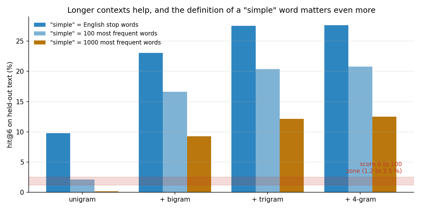
The organisers' notebook outputs the and five dummy words: since the can never be the answer, it scores 0. The simplest real model is the unigram one: always propose the six most frequent non-simple words (harry, said, ron...). If "simple" means English stop words, it already hits 9.8 % of our validation positions; if "simple" means the 100 most frequent words, it hits 2.1 %; if it means the 1000 most frequent words, 0.15 %.

Since the official thresholds are 1.2 % and 2.5 %, a unigram model on the hidden test must sit near or below 1.2 %. This strongly suggests that the hidden words are rare words, closer to our strictest definition: keep that in mind when reading validation numbers, which are certainly optimistic.

The key idea

A language model estimates $P(w \mid \text{context})$. With counts, the maximum-likelihood estimate given the last $n$ words is

$$P_n(w \mid c_n) = \frac{\#(c_n\, w)}{\#(c_n\, \cdot)} ,$$

where $c_n$ is the context of length $n$. Long contexts are precise but rarely seen (only 24 % of the test lines end with a trigram that appears in the library); short contexts are always available but vague. Interpolation combines them:

$$\text{score}(w) = \sum_{n=0}^{3} \lambda_n\, P_n(w \mid c_n), \qquad \lambda = (0.05,\ 1,\ 2,\ 4),$$

with increasing weights, so a seen long context dominates and the shorter ones take over when it was never seen. (This is a simple cousin of Jelinek-Mercer smoothing and of the "stupid backoff" used in early web-scale models.)

The second idea is about the constraint in the statement: the hidden word is never simple, so we condition on it. We count only non-simple next words, which means

$$P(w \mid c, \text{not simple}) = \frac{P(w\mid c)}{P(\text{not simple}\mid c)} \text{ for non-simple } w,$$

and the six guesses are never wasted on the, of or and. On our validation set this alone raises hit@6 from 21.3 % to 27.7 % (stop-word definition): when the context is "he looked at the", a plain model would happily spend guesses on function words.

The full solution

1. Read the library, replace the ligatures in the test text, split on spaces.
2. For $n = 0, 1, 2, 3$, count which non-simple words follow each context of length $n$ (a dictionary from tuples of words to Counters). We use scikit-learn's English stop-word list as the "simple" words.
3. For each test line, add up $\lambda_n P_n(w\mid c_n)$ over the 50 most frequent continuations of each context, keep the 6 best, and pad with the most frequent words if fewer than 6 candidates exist.
4. Print six lines word score and an empty line per test case, as in the organisers' notebook.

for n, lam in enumerate(LAMBDA):
    c = tabs[n].get(tuple(ctx[len(ctx) - n:]))   # continuations of the last n words
    if c:
        tot = sum(c.values())
        for w, v in c.most_common(50):
            score[w] += lam * v / tot

The whole thing runs in a few seconds; the predictions are then printed by the submitted program.

Results

hit@6 on 4000 random validation positions in the held-out last 10 % of the library:

approach	simple = stop words	simple = top-100 words	simple = top-1000 words
organisers' notebook (the + dummies)	0 %	0 %	0 %
unigram (6 most frequent non-simple words)	9.8 %	2.1 %	0.15 %
+ bigram	23.1 %	16.7 %	9.3 %
+ trigram	27.5 %	20.4 %	12.2 %
+ 4-gram (final)	27.7 %	20.8 %	12.5 %
4-gram without removing simple words from the counts	21.3 %
equal weights $\lambda = (0.05, 1, 1, 1)$	27.8 %

Even excluding the 3000 most frequent words, the final model hits 11.1 % (the unigram: 0 %). Every variant is far above 2.5 %, so on our validation the score is capped at 100. We cannot claim the same on the hidden test: the low official thresholds mean the hidden words are much harder than ours (rarer words, and a different book), and the honest conclusion is "our validation is too easy to calibrate the final score". What we can say is that the ranking of the methods is the same under every definition of "simple" we tried, and that a context of 3 words captures nearly all of the gain (the 4-gram adds almost nothing because 4-word contexts are rarely seen twice).

What to remember

• Interpolate n-gram orders: long contexts are precise but sparse, short ones are robust; a weighted sum gets the best of both.
• Use every constraint the statement gives you. "The word is not simple" is information: conditioning on it gave +6 points of hit@6.
• Look at the raw test text. Two invisible ligature characters would have silently broken every context that contains them.
• Question your validation set. If a trivial baseline already beats the official "best" threshold on your validation, your validation does not look like the test; say so rather than trusting the number.
• Counting is a language model. Before neural networks, this is how $P(\text{next word} \mid \text{context})$ was estimated, and it remains a strong, instant baseline.